Problem Set 6#
See Merge, Reshape, and GroupBy
import matplotlib.pyplot as plt
import numpy as np
import pandas as pd

%matplotlib inline
Questions 1-7#
Lets start with a relatively straightforward exercise before we get to the really fun stuff.
The following code loads a cleaned piece of census data from Statistics Canada.
df = pd.read_csv("https://datascience.quantecon.org/assets/data/canada_census.csv", header=0, index_col=False)
df.head()
| CDcode | Pname | Population | CollegeEducated | PercentOwnHouse | Income | |
|---|---|---|---|---|---|---|
| 0 | 1001 | Newfoundland and Labrador | 270350 | 24.8 | 74.1 | 74676 |
| 1 | 1002 | Newfoundland and Labrador | 20370 | 7.5 | 86.3 | 60912 |
| 2 | 1003 | Newfoundland and Labrador | 15560 | 7.3 | 86.0 | 56224 |
| 3 | 1004 | Newfoundland and Labrador | 20385 | 10.9 | 73.7 | 44282 |
| 4 | 1005 | Newfoundland and Labrador | 42015 | 17.0 | 73.9 | 62565 |
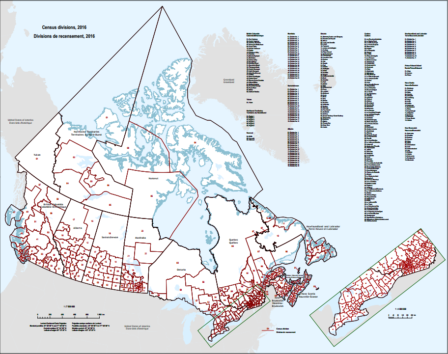
A census division is a geographical area, smaller than a Canadian province, that is used to organize information at a slightly more granular level than by province or by city. The census divisions are shown below.
The data above contains information on the population, percent of population with a college degree, percent of population who own their house/apartment, and the median after-tax income at the census division level.
Hint: The groupby is the key here. You will need to practice different split, apply, and combine options.
Question 1#
Assume that you have a separate data source with province codes and names.
df_provincecodes = pd.DataFrame({
    "Pname" : [ 'Newfoundland and Labrador', 'Prince Edward Island', 'Nova Scotia',
                'New Brunswick', 'Quebec', 'Ontario', 'Manitoba', 'Saskatchewan',
                'Alberta', 'British Columbia', 'Yukon', 'Northwest Territories','Nunavut'],
    "Code" : ['NL', 'PE', 'NS', 'NB', 'QC', 'ON', 'MB', 'SK', 'AB', 'BC', 'YT', 'NT', 'NU']
            })
df_provincecodes
| Pname | Code | |
|---|---|---|
| 0 | Newfoundland and Labrador | NL |
| 1 | Prince Edward Island | PE |
| 2 | Nova Scotia | NS |
| 3 | New Brunswick | NB |
| 4 | Quebec | QC |
| 5 | Ontario | ON |
| 6 | Manitoba | MB |
| 7 | Saskatchewan | SK |
| 8 | Alberta | AB |
| 9 | British Columbia | BC |
| 10 | Yukon | YT |
| 11 | Northwest Territories | NT |
| 12 | Nunavut | NU |
With this,
Either merge or join these province codes into the census dataframe to provide province codes for each province name. Hint: You need to figure out which “key” matches in the merge, and don’t be afraid to rename columns for convenience.
Drop the province names from the resulting dataframe.
Rename the column with the province codes to “Province”. Hint:
.rename(columns = <YOURDICTIONARY>)
# Your code here
For this particular example, you could have renamed the column using replace. This is a good check.
(pd.read_csv("https://datascience.quantecon.org/assets/data/canada_census.csv", header=0, index_col=False)
.replace({
    "Alberta": "AB", "British Columbia": "BC", "Manitoba": "MB", "New Brunswick": "NB",
    "Newfoundland and Labrador": "NL", "Northwest Territories": "NT", "Nova Scotia": "NS",
    "Nunavut": "NU", "Ontario": "ON", "Prince Edward Island": "PE", "Quebec": "QC",
    "Saskatchewan": "SK", "Yukon": "YT"})
.rename(columns={"Pname" : "Province"})
.head()
)
| CDcode | Province | Population | CollegeEducated | PercentOwnHouse | Income | |
|---|---|---|---|---|---|---|
| 0 | 1001 | NL | 270350 | 24.8 | 74.1 | 74676 |
| 1 | 1002 | NL | 20370 | 7.5 | 86.3 | 60912 |
| 2 | 1003 | NL | 15560 | 7.3 | 86.0 | 56224 |
| 3 | 1004 | NL | 20385 | 10.9 | 73.7 | 44282 |
| 4 | 1005 | NL | 42015 | 17.0 | 73.9 | 62565 |
Question 2#
Which province has the highest population? Which has the lowest?
# Your code here
Question 3#
Show a bar plot and a pie plot of the province populations. Hint: After the split-apply-combine, you can use .plot.bar() or .plot.pie().
# Your code here
Question 3#
Which province has the highest percent of individuals with a college education? Which has the lowest?
Hint: Remember to weight this calculation by population!
# Your code here
Question 4#
What is the census division with the highest median income in each province?
# Your code here
Question 5#
By province, what is the total population of census divisions where more than 80 percent of the population own houses ?
# Your code here
Question 6#
By province, what is the average proportion of college-educated individuals in census divisions where more than 80 percent of the population own houses?
# Your code here
Question 7#
Classify the census divisions as low, medium, and highly-educated by using the college-educated proportions, where “low” indicates that less than 10 percent of the area is college-educated, “medium” indicates between 10 and 20 percent is college-educated, and “high” indicates more than 20 percent.
Based on that classification, find the average median income across census divisions for each category.
# Your code here
Questions 8-9#
Let’s look at another example.
This time, we will use a dataset from the Bureau of Transportation Statistics that describes the cause for all US domestic flight delays in November 2016:
Loading this dataset the first time will take a minute or two because it is quite hefty… We recommend taking a break to view this xkcd comic.
url = "https://datascience.quantecon.org/assets/data/airline_performance_dec16.csv.zip"
air_perf = pd.read_csv(url)[["CRSDepTime", "Carrier", "CarrierDelay", "ArrDelay"]]
air_perf.info()
air_perf.head()
<class 'pandas.core.frame.DataFrame'>
RangeIndex: 460949 entries, 0 to 460948
Data columns (total 4 columns):
 #   Column        Non-Null Count   Dtype
---  ------        --------------   -----
 0   CRSDepTime    460949 non-null  object
 1   Carrier       460949 non-null  object
 2   CarrierDelay  460949 non-null  float64
 3   ArrDelay      452229 non-null  float64
dtypes: float64(2), object(2)
memory usage: 14.1+ MB
| CRSDepTime | Carrier | CarrierDelay | ArrDelay | |
|---|---|---|---|---|
| 0 | 2016-12-18 15:58:00 | AA | 0.0 | 20.0 |
| 1 | 2016-12-19 15:58:00 | AA | 0.0 | 20.0 |
| 2 | 2016-12-20 15:58:00 | AA | 0.0 | -3.0 |
| 3 | 2016-12-21 15:58:00 | AA | 0.0 | -10.0 |
| 4 | 2016-12-22 15:58:00 | AA | 0.0 | -8.0 |
The Carrier column identifies the airline while the CarrierDelay
reports the total delay, in minutes, that was the “carrier’s fault”.
Question 8#
Determine the 10 airlines which, on average, contribute most to delays.
# Your code here
# avg_delays =
Question 9#
One issue with this dataset is that we might not know what all those two letter carrier codes are!
Thankfully, we have a second dataset that maps two-letter codes to full airline names:
url = "https://datascience.quantecon.org/assets/data/airline_carrier_codes.csv.zip"
carrier_code = pd.read_csv(url)
carrier_code.tail()
| Code | Description | |
|---|---|---|
| 1884 | ZW | Air Wisconsin Airlines Corp (1994 - ) |
| 1885 | ZX | Airbc Ltd. (1990 - 2000) |
| 1886 | ZX | Air Georgian (2002 - ) |
| 1887 | ZY | Atlantic Gulf Airlines (1985 - 1986) |
| 1888 | ZYZ | Skyway Aviation Inc. (1960 - 2002) |
In this question, you should merge the carrier codes and the previously computed dataframe from Question 9 (the 10 airlines that contribute most to delays).
# Your code here
# avg_delays_w_name
Question 10#
In this question, we will load data from the World Bank. World Bank data is often stored in formats containing vestigial columns because of their data format standardization.
This particular data contains the world’s age dependency ratios (old) across countries. The ratio is the number of people who are above 65 divided by the number of people between 16 and 65 and measures how many working individuals exist relative to the number of dependent (retired) individuals.
adr = pd.read_csv("https://datascience.quantecon.org/assets/data/WorldBank_AgeDependencyRatio.csv")
adr.head()
| Series Name | Series Code | Country Name | Country Code | 1960 | 1970 | 1980 | 1990 | 2000 | 2010 | 2017 | |
|---|---|---|---|---|---|---|---|---|---|---|---|
| 0 | Age dependency ratio, old (% of working-age po... | SP.POP.DPND.OL | Belgium | BEL | 18.376221914997 | 21.3310651174022 | 22.0827795865161 | 22.3478876919412 | 25.7237772053865 | 26.3502220937405 | 28.8663095376732 |
| 1 | Age dependency ratio, old (% of working-age po... | SP.POP.DPND.OL | High income | HIC | 13.7442735255142 | 15.5128071607608 | 17.2793259853973 | 18.1810594950547 | 20.238646358909 | 22.5821690792651 | 26.5545126329423 |
| 2 | Age dependency ratio, old (% of working-age po... | SP.POP.DPND.OL | Andorra | AND | .. | .. | .. | .. | .. | .. | .. |
| 3 | Age dependency ratio, old (% of working-age po... | SP.POP.DPND.OL | Austria | AUT | 18.5196085788113 | 22.7370767160537 | 23.6381357233154 | 21.8956152694877 | 22.7046805297879 | 26.373860988558 | 28.7849528312483 |
| 4 | Age dependency ratio, old (% of working-age po... | SP.POP.DPND.OL | Bermuda | BMU | .. | .. | .. | .. | .. | .. | .. |
This data only has a single variable, so you can eliminate the Series Name and Series Code
columns. You can also eliminate the Country Code or Country Name column (but not both),
since they contain repetitive information.
We can organize this data in a couple of ways.
The first (and the one we’d usually choose) is to place the years and country names on the index and have a single column. (If we had more variables, each variable could have its own column.)
Another reasonable organization is to have one country per column and place the years on the index.
Your goal is to reshape the data both ways. Which is easier? Which do you think a better organization method?
# Reshape to have years and countries on index
# Reshape to have years on index and country identifiers as columns