Machine Learning in Economics#
Author
Prerequisites
Outcomes
Understand how economists use machine learning in academic research
# Uncomment following line to install on colab
#! pip install fiona geopandas xgboost gensim folium pyLDAvis descartes
import matplotlib.pyplot as plt
import numpy as np
import pandas as pd


%matplotlib inline
#plt.style.use('tableau-colorblind10')
#plt.style.use('Solarize_Light2')
plt.style.use('bmh')
Introduction#
Machine learning is increasingly being utilized in economic research. Here, we discuss three main ways that economists are currently using machine learning methods.
Prediction Policy#
Most empirical economic research focuses on questions of causality. However, machine learning methods can actually be used in economic research or policy making when the goal is prediction.
[mlKLMO15] is a short paper which makes this point.
Consider two toy examples. One policymaker facing a drought must decide whether to invest in a rain dance to increase the chance of rain. Another seeing clouds must decide whether to take an umbrella to work to avoid getting wet on the way home. Both decisions could benefit from an empirical study of rain. But each has differ-ent requirements of the estimator. One requires causality: Do rain dances cause rain? The other does not, needing only prediction: Is the chance of rain high enough to merit an umbrella? We often focus on rain dance–like policy problems. But there are also many umbrella-like policy problems. Not only are these prediction problems neglected, machine learning can help us solve them more effectively. [mlKLMO15].
One of their examples is the allocation of joint replacements for osteoarthritis in elderly patients. Joint replacements are costly, both monetarily and in terms of potentially painful recovery from surgery. Joint replacements may not be worthwhile for patients who do not live long enough afterward to enjoy the benefits. [mlKLMO15] uses machine learning methods to predict mortality and argues that avoiding joint replacements for people with the highest predicted mortality risk could lead to sizable benefits.
Other situations where improved prediction could improve economic policy include:
Targeting safety or health inspections.
Predicting highest risk youth for targeting interventions.
Improved risk scoring in insurance markets to reduce adverse selection.
Improved credit scoring to better allocate credit.
Predicting the risk someone accused of a crime does not show up for trial to help decide whether to offer bail [mlKLL+17].
We investigated one such prediction policy problem in recidivism.
Estimation of Nuisance Functions#
Most empirical economic studies are interested in a single low dimensional parameter, but determining that parameter may require estimating additional “nuisance” parameters to estimate this coefficient consistently and avoid omitted variables bias. However, the choice of which other variables to include and their functional forms is often somewhat arbitrary. One promising idea is to use machine learning methods to let the data decide what control variables to include and how. Care must be taken when doing so, though, because machine learning’s flexibility and complexity – what make it so good at prediction – also pose challenges for inference.
Partially Linear Regression#
To be more concrete, consider a regression model. We have some regressor of interest, \(d\), and we want to estimate the effect of \(d\) on \(y\). We have a rich enough set of controls \(x\) that we are willing to believe that \(E[\epsilon|d,x] = 0\) . \(d_i\) and \(y_i\) are scalars, while \(x_i\) is a vector. We are not interested in \(x\) per se, but we need to include it to avoid omitted variable bias. Suppose the true model generating the data is:
where \(f(x)\) is some unknown function. This is called a partially linear model: linear in \(d\), but not in \(x\) .
A typical applied econometric approach for this model would be to choose some transform of \(x\), say \(X = T(x)\), where \(X\) could be some subset of \(x\) , perhaps along with interactions, powers, and so on. Then, we estimate a linear regression,
and then perhaps also report results for a handful of different choices of \(T(x)\) .
Some downsides to the typical applied econometric practice include:
The choice of \(T\) is arbitrary, which opens the door to specification searching and p-hacking.
If \(x\) is high dimensional and \(X\) is low dimensional, a poor choice will lead to omitted variable bias. Even if \(x\) is low dimensional, omitted variable bias occurs if \(f(x)\) is poorly approximated by \(X'\beta\).
In some sense, machine learning can be thought of as a way to choose \(T\) in an automated and data-driven way. Choosing which machine learning method to use and tuning parameters specifically for that method are still potentially arbitrary decisions, but these decisions may have less impact.
Economic researchers typically don’t just want an estimate of \(\theta\), \(\hat{\theta}\). Instead, they want to know that \(\hat{\theta}\) has good statistical properties (it should at least be consistent), and they want some way to quantify how uncertain is \(\hat{\theta}\) (i.e. they want a standard error). The complexity of machine learning methods makes their statistical properties difficult to understand. If we want \(\hat{\theta}\) to have known and good statistical properties, we must make sure we use machine learning methods correctly. A procedure to estimate \(\theta\) in the partially linear model is as follows:
Predict \(y\) and \(d\) from \(x\) using any machine learning method with “cross-fitting”.
Partition the data in \(k\) subsets.
For the \(j\) th subset, train models to predict \(y\) and \(d\) using the other \(k-1\) subsets. Denote the predictions from these models as \(p^y_{-j}(x)\) and \(p^d_{-j}(x)\).
For \(y_i\) in the \(j\) -th subset use the other \(k-1\) subsets to predict \(\hat{y}_i = p^y_{-j(i)}(x_i)\)
Partial out \(x\) : let \(\tilde{y}_i = y_i - \hat{y}_i\) and \(\tilde{d}_i = d_i - \hat{d}_i\).
Regress \(\tilde{y}_i\) on \(\tilde{d}_i\), let \(\hat{\theta}\) be the estimated coefficient for \(\tilde{d}_i\) . \(\hat{\theta}\) is consistent, asymptotically normal, and has the usual standard error (i.e. the standard error given by statsmodels is correct).
Some remarks:
This procedure gives a \(\hat{\theta}\) that has the same asymptotic distribution as what we would get if we knew the true \(f(x)\) . In statistics, we call this an oracle property, because it is as if an all knowing oracle told us \(f(x)\).
This procedure requires some technical conditions on the data-generating process and machine learning estimator, but we will not worry about them here. See [mlCCD+18] for details.
Here is code implementing the above idea.
from sklearn.model_selection import cross_val_predict
from sklearn import linear_model
import statsmodels as sm

def partial_linear(y, d, X, yestimator, destimator, folds=3):
    """Estimate the partially linear model y = d*C + f(x) + e

    Parameters
    ----------
    y : array_like
        vector of outcomes
    d : array_like
        vector or matrix of regressors of interest
    X : array_like
        matrix of controls
    mlestimate : Estimator object for partialling out X. Must have ‘fit’
        and ‘predict’ methods.
    folds : int
        Number of folds for cross-fitting

    Returns
    -------
    ols : statsmodels regression results containing estimate of coefficient on d.
    yhat : cross-fitted predictions of y
    dhat : cross-fitted predictions of d
    """

    # we want predicted probabilities if y or d is discrete
    ymethod = "predict" if False==getattr(yestimator, "predict_proba",False) else "predict_proba"
    dmethod = "predict" if False==getattr(destimator, "predict_proba",False) else "predict_proba"
    # get the predictions
    yhat = cross_val_predict(yestimator,X,y,cv=folds,method=ymethod)
    dhat = cross_val_predict(destimator,X,d,cv=folds,method=dmethod)
    ey = np.array(y - yhat)
    ed = np.array(d - dhat)
    ols = sm.regression.linear_model.OLS(ey,ed).fit(cov_type='HC0')

    return(ols, yhat, dhat)
Application: Gender Wage Gap#
Okay, enough theory. Let’s look at an application. Policy makers have long been concerned with the gender wage gap. We will examine the gender wage gap using data from the 2018 Current Population Survey (CPS) in the US. In particular, we will use the version of the CPS provided by the NBER.
import statsmodels.formula.api as smf
from statsmodels.iolib.summary2 import summary_col
# Download CPS data
cpsall = pd.read_stata("https://www.nber.org/morg/annual/morg18.dta")

# take subset of data just to reduce computation time
cps = cpsall.sample(30000, replace=False, random_state=0)
display(cps.head())
cps.describe()
| hhid | intmonth | hurespli | hrhtype | minsamp | hrlonglk | hrsample | hrhhid2 | serial | hhnum | ... | ym_file | ym | ch02 | ch35 | ch613 | ch1417 | ch05 | ihigrdc | docc00 | dind02 | |
|---|---|---|---|---|---|---|---|---|---|---|---|---|---|---|---|---|---|---|---|---|---|
| 103153 | 150909100105603 | May | 1.0 | Civilian male primary individual | MIS 4 | MIS 2-4 Or MIS 6-8 (link To | 0801 | 08011 | 1 | 1 | ... | 700 | 697 | 0 | 0 | 0 | 0 | 0 | NaN | Business and financial operations occupations | Professional and Technical services |
| 76648 | 505760912076673 | March | 1.0 | Husband/wife primary fam (neither in Armed For... | MIS 4 | MIS 2-4 Or MIS 6-8 (link To | 0811 | 08111 | 1 | 1 | ... | 698 | 695 | 0 | 0 | 0 | 0 | 0 | 12.0 | NaN | NaN |
| 51433 | 481462012350753 | February | 1.0 | Husband/wife primary fam (neither in Armed For... | MIS 4 | MIS 2-4 Or MIS 6-8 (link To | 0701 | 07011 | 1 | 1 | ... | 697 | 694 | 0 | 0 | 0 | 0 | 0 | NaN | Management occupations | Agriculture |
| 75550 | 106518879410166 | March | 2.0 | Husband/wife primary fam (neither in Armed For... | MIS 8 | MIS 2-4 Or MIS 6-8 (link To | 0611 | 06111 | 1 | 1 | ... | 698 | 683 | 0 | 0 | 0 | 0 | 0 | 11.0 | NaN | NaN |
| 284643 | 466023401171104 | December | 1.0 | Husband/wife primary fam (neither in Armed For... | MIS 4 | MIS 2-4 Or MIS 6-8 (link To | 0901 | 09011 | 1 | 1 | ... | 707 | 704 | 0 | 1 | 1 | 0 | 1 | 13.0 | Management occupations | Membership associations and organizations |
5 rows × 98 columns
| hurespli | hhnum | cbsafips | county | centcity | smsastat | icntcity | smsa04 | relref95 | age | ... | recnum | year | ym_file | ym | ch02 | ch35 | ch613 | ch1417 | ch05 | ihigrdc | |
|---|---|---|---|---|---|---|---|---|---|---|---|---|---|---|---|---|---|---|---|---|---|
| count | 29997.000000 | 30000.000000 | 30000.000000 | 30000.000000 | 24701.000000 | 29689.000000 | 3845.000000 | 30000.000000 | 30000.000000 | 30000.000000 | ... | 30000.00000 | 30000.0 | 30000.000000 | 30000.000000 | 30000.00000 | 30000.000000 | 30000.000000 | 30000.000000 | 30000.000000 | 21463.000000 |
| mean | 1.314898 | 1.052733 | 22812.328667 | 25.752033 | 1.926157 | 1.188150 | 1.377373 | 3.687667 | 3.200333 | 47.856967 | ... | 217052.62500 | 2018.0 | 701.467433 | 692.357833 | 0.06040 | 0.065333 | 0.143033 | 0.086467 | 0.105033 | 12.355938 |
| std | 0.683163 | 0.245943 | 16494.302775 | 62.862911 | 0.721596 | 0.390839 | 0.946464 | 2.592477 | 3.291772 | 18.757968 | ... | 125652.34375 | 0.0 | 3.467921 | 6.970577 | 0.23823 | 0.247117 | 0.350113 | 0.281057 | 0.306601 | 2.478719 |
| min | 0.000000 | 1.000000 | 0.000000 | 0.000000 | 1.000000 | 1.000000 | 1.000000 | 0.000000 | 1.000000 | 16.000000 | ... | 19.00000 | 2018.0 | 696.000000 | 681.000000 | 0.00000 | 0.000000 | 0.000000 | 0.000000 | 0.000000 | 0.000000 |
| 25% | 1.000000 | 1.000000 | 0.000000 | 0.000000 | 1.000000 | 1.000000 | 1.000000 | 0.000000 | 1.000000 | 32.000000 | ... | 108185.25000 | 2018.0 | 698.000000 | 686.000000 | 0.00000 | 0.000000 | 0.000000 | 0.000000 | 0.000000 | 12.000000 |
| 50% | 1.000000 | 1.000000 | 25420.000000 | 0.000000 | 2.000000 | 1.000000 | 1.000000 | 4.000000 | 2.000000 | 48.000000 | ... | 217388.50000 | 2018.0 | 701.000000 | 692.000000 | 0.00000 | 0.000000 | 0.000000 | 0.000000 | 0.000000 | 12.000000 |
| 75% | 1.000000 | 1.000000 | 37900.000000 | 29.000000 | 2.000000 | 1.000000 | 1.000000 | 6.000000 | 3.000000 | 63.000000 | ... | 325915.00000 | 2018.0 | 704.000000 | 698.000000 | 0.00000 | 0.000000 | 0.000000 | 0.000000 | 0.000000 | 14.000000 |
| max | 11.000000 | 8.000000 | 49740.000000 | 810.000000 | 3.000000 | 2.000000 | 7.000000 | 7.000000 | 18.000000 | 85.000000 | ... | 434279.00000 | 2018.0 | 707.000000 | 704.000000 | 1.00000 | 1.000000 | 1.000000 | 1.000000 | 1.000000 | 18.000000 |
8 rows × 62 columns
The variable “earnwke” records weekly earnings. Two variables detail the hours of work. “uhours” is usual hours worked per week, and “hourslw” is hours worked last week. We will try using each measure of hours to construct the wage. Let’s estimate the unconditional gender earnings and wage gaps.
cps["female"] = (cps.sex==2)
cps["log_earn"] = np.log(cps.earnwke)
cps.loc[np.isinf(cps.log_earn),"log_earn"] = np.nan
cps["log_uhours"] = np.log(cps.uhourse)
cps.loc[np.isinf(cps.log_uhours),"log_uhours"] = np.nan
cps["log_hourslw"] = np.log(cps.hourslw)
cps.loc[np.isinf(cps.log_hourslw),"log_hourslw"] = np.nan
cps["log_wageu"] = cps.log_earn - cps.log_uhours
cps["log_wagelw"] = cps.log_earn - cps.log_hourslw


lm = list()
lm.append(smf.ols(formula="log_earn ~ female", data=cps,
                  missing="drop").fit(cov_type='HC0'))
lm.append( smf.ols(formula="log_wageu ~ female", data=cps,
                   missing="drop").fit(cov_type='HC0'))
lm.append(smf.ols(formula="log_wagelw ~ female", data=cps,
                  missing="drop").fit(cov_type='HC0'))
lm.append(smf.ols(formula="log_earn ~ female + log_hourslw + log_uhours", data=cps,
                  missing="drop").fit(cov_type='HC0'))
Show code cell output
/home/runner/miniconda3/envs/lecture-datascience/lib/python3.12/site-packages/pandas/core/arraylike.py:399: RuntimeWarning: divide by zero encountered in log
  result = getattr(ufunc, method)(*inputs, **kwargs)
/home/runner/miniconda3/envs/lecture-datascience/lib/python3.12/site-packages/pandas/core/arraylike.py:399: RuntimeWarning: divide by zero encountered in log
  result = getattr(ufunc, method)(*inputs, **kwargs)
/home/runner/miniconda3/envs/lecture-datascience/lib/python3.12/site-packages/pandas/core/arraylike.py:399: RuntimeWarning: invalid value encountered in log
  result = getattr(ufunc, method)(*inputs, **kwargs)
summary_col(lm, stars=True)
| log_earn I | log_wageu I | log_wagelw I | log_earn II | |
|---|---|---|---|---|
| Intercept | 6.7473*** | 3.0970*** | 3.1056*** | 1.8014*** |
| (0.0088) | (0.0072) | (0.0078) | (0.0933) | |
| female[T.True] | -0.3004*** | -0.1695*** | -0.1707*** | -0.1258*** |
| (0.0127) | (0.0102) | (0.0112) | (0.0105) | |
| log_hourslw | 0.0907*** | |||
| (0.0285) | ||||
| log_uhours | 1.2631*** | |||
| (0.0431) | ||||
| R-squared | 0.0338 | 0.0179 | 0.0149 | 0.4139 |
| R-squared Adj. | 0.0337 | 0.0179 | 0.0148 | 0.4137 |
Standard errors in parentheses.
* p<.1, ** p<.05, ***p<.01
The unconditional gender gap in log earnings is about -0.3. Women earn about 30% less than men. The unconditional gender wage gap is about 18%. The last column gives the gender earnings gap conditional on hours. This could differ from the wage gap if, for example, full time workers are paid higher wages than part-time. Some evidence has suggested this, and the gender earnings gap conditional on hours is about 15%.
Equal Pay for Equal Work?#
A common slogan is equal pay for equal work. One way to interpret this is that for employees with similar worker and job characteristics, no gender wage gap should exist.
Eliminating this wage gap across similar worker and job characteristics is one necessary (though insufficient) condition for equality. Some of the differences (like hours in the 4th column of the above table) might actually be a result of societal norms and/or discrimination, so we don’t want to overgeneralize.
Nonetheless, let’s examine whether there is a gender wage gap conditional on all worker and job characteristics. We want to ensure that we control for those characteristics as flexibly as possible, so we will use the partially linear model described above.
from patsy import dmatrices
# Prepare data
fmla  = "log_earn + female ~ log_uhours + log_hourslw + age + I(age**2) + C(race) + C(cbsafips) + C(smsastat) + C(grade92) + C(unionmme) + C(unioncov) + C(ind02) + C(occ2012)"
yd, X = dmatrices(fmla,cps)
female = yd[:,1]
logearn = yd[:,2]
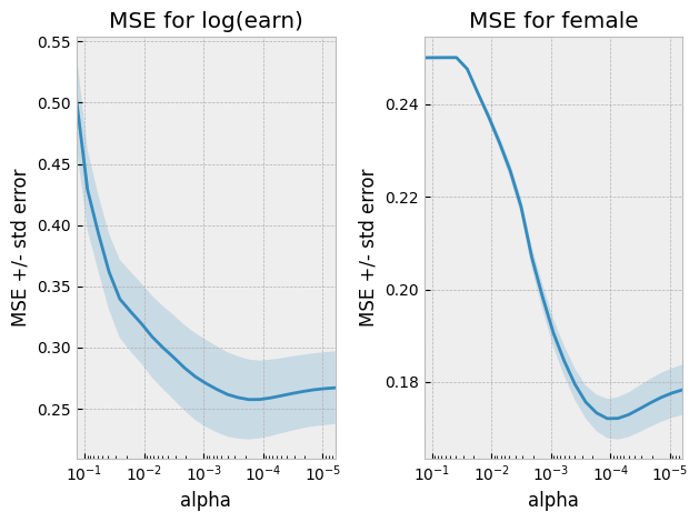
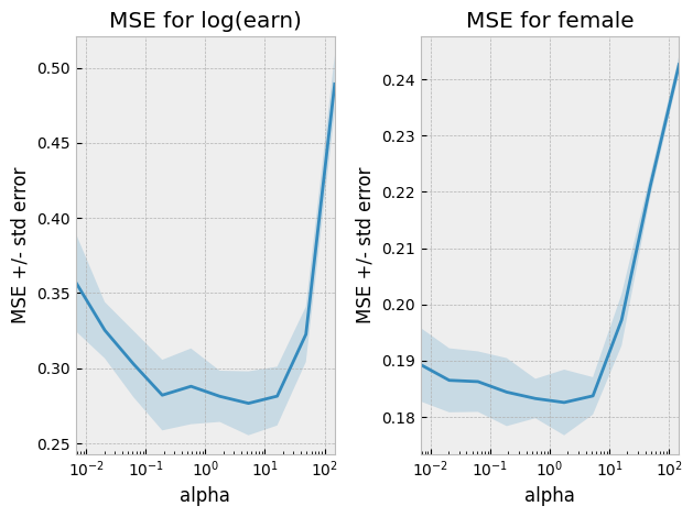
The choice of regularization parameter is somewhat tricky. Cross-validation is a good way to choose the best regularization parameter when our goal is prediction. However, our goal here is not prediction. Instead, we want to get a well-behaved estimate of the gender wage gap. To achieve this, we generally need a smaller regularization parameter than what would minimize MSE. The following code picks such a regularization parameter. Note however, that the details of this code might not meet the technical theoretical conditions needed for our ultimate estimate of the gender wage gap to be consistent and asymptotically normal. The R package, “HDM” [mlCHS16] , chooses the regularization parameter in way that is known to be correct.
# select regularization parameter
alphas = np.exp(np.linspace(-2, -12, 25))
lassoy = linear_model.LassoCV(cv=6, alphas=alphas, max_iter=5000).fit(X,logearn)
lassod = linear_model.LassoCV(cv=6, alphas=alphas, max_iter=5000).fit(X,female)
fig, ax = plt.subplots(1,2)

def plotlassocv(l, ax) :
    alphas = l.alphas_
    mse = l.mse_path_.mean(axis=1)
    std_error = l.mse_path_.std(axis=1)
    ax.plot(alphas,mse)
    ax.fill_between(alphas, mse + std_error, mse - std_error, alpha=0.2)

    ax.set_ylabel('MSE +/- std error')
    ax.set_xlabel('alpha')
    ax.set_xlim([alphas[0], alphas[-1]])
    ax.set_xscale("log")
    return(ax)

ax[0] = plotlassocv(lassoy,ax[0])
ax[0].set_title("MSE for log(earn)")
ax[1] = plotlassocv(lassod,ax[1])
ax[1].set_title("MSE for female")
fig.tight_layout()

# there are theoretical reasons to choose a smaller regularization
# than the one that minimizes cv. BUT THIS WAY OF CHOOSING IS ARBITRARY AND MIGHT BE WRONG
def pickalpha(lassocv) :
    imin = np.argmin(lassocv.mse_path_.mean(axis=1))
    msemin = lassocv.mse_path_.mean(axis=1)[imin]
    se = lassocv.mse_path_.std(axis=1)[imin]
    alpha= min([alpha for (alpha, mse) in zip(lassocv.alphas_, lassocv.mse_path_.mean(axis=1)) if mse<msemin+se])
    return(alpha)

alphay = pickalpha(lassoy)
alphad = pickalpha(lassod)
# show results
pl_lasso = partial_linear(logearn, female, X,
                          linear_model.Lasso(alpha=lassoy.alpha_),
                          linear_model.Lasso(alpha=lassod.alpha_))
pl_lasso[0].summary()
| Dep. Variable: | y | R-squared (uncentered): | 0.009 |
|---|---|---|---|
| Model: | OLS | Adj. R-squared (uncentered): | 0.009 |
| Method: | Least Squares | F-statistic: | 107.2 |
| Date: | Wed, 05 Feb 2025 | Prob (F-statistic): | 4.91e-25 |
| Time: | 03:44:19 | Log-Likelihood: | -9718.3 |
| No. Observations: | 13052 | AIC: | 1.944e+04 |
| Df Residuals: | 13051 | BIC: | 1.945e+04 |
| Df Model: | 1 | ||
| Covariance Type: | HC0 |
| coef | std err | z | P>|z| | [0.025 | 0.975] | |
|---|---|---|---|---|---|---|
| x1 | -0.1160 | 0.011 | -10.356 | 0.000 | -0.138 | -0.094 |
| Omnibus: | 6939.182 | Durbin-Watson: | 1.959 |
|---|---|---|---|
| Prob(Omnibus): | 0.000 | Jarque-Bera (JB): | 410073.398 |
| Skew: | -1.777 | Prob(JB): | 0.00 |
| Kurtosis: | 30.229 | Cond. No. | 1.00 |
Notes:
[1] R² is computed without centering (uncentered) since the model does not contain a constant.
[2] Standard Errors are heteroscedasticity robust (HC0)
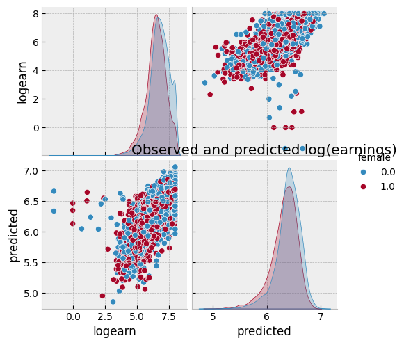
import seaborn as sns
# Visualize predictions
def plotpredictions(pl) :
df = pd.DataFrame({"logearn":logearn,
"predicted":pl[1],
"female":female,
"P(female|x)":pl[2]})
sns.pairplot(df, vars=["logearn","predicted"], hue="female")
plt.title("Observed and predicted log(earnings)")
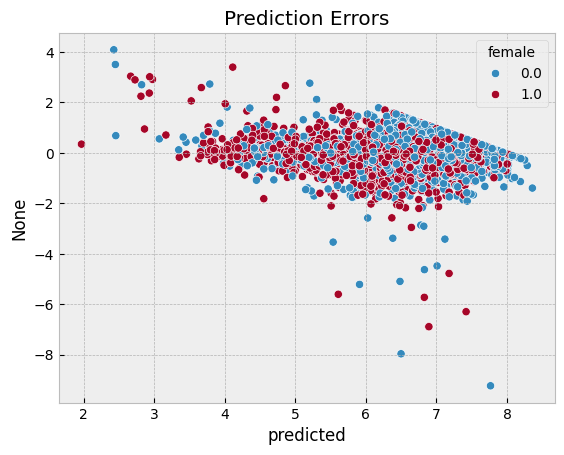
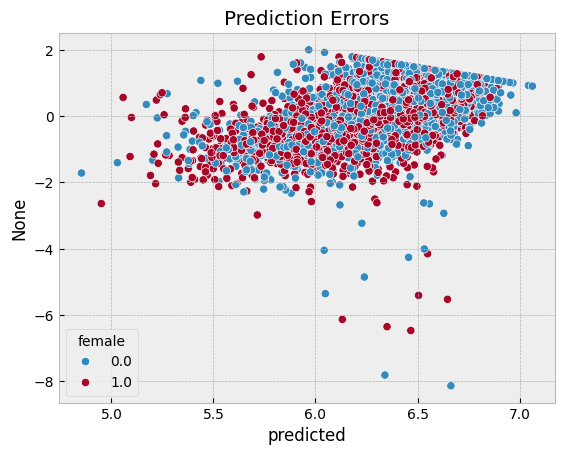
plt.figure()
sns.scatterplot(x = df.predicted, y = df.logearn-df.predicted, hue=df.female)
plt.title("Prediction Errors")
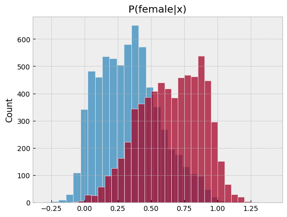
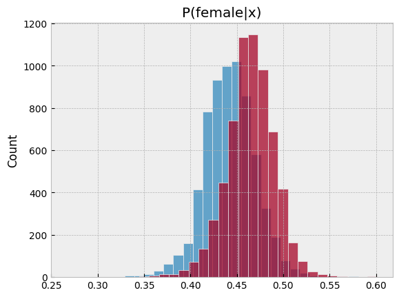
plt.figure()
sns.histplot(pl[2][female == 0], bins=30, label="Male", kde=False)
sns.histplot(pl[2][female == 1], bins=30, label="Female", kde=False)
plt.title('P(female|x)')
plotpredictions(pl_lasso)
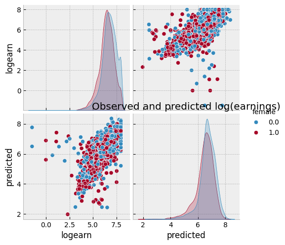
We see that the gender earnings gap is 12.4%, conditional on hours, age, race, location, education, union membership, industry, and occupation. Compared to the gap conditional on only hours, differences in other observable characteristics in the CPS seem unable explain much of the gender earnings gap.
We can repeat the same procedure with another machine learning method in place of lasso. Let’s try it with neural networks.
from sklearn import neural_network
from sklearn import preprocessing, pipeline, model_selection

nnp = pipeline.Pipeline(steps=[
    ("scaling", preprocessing.StandardScaler()),
    ("nn", neural_network.MLPRegressor((50,), activation="logistic",
                                       verbose=False, solver="adam",
                                       max_iter=400, early_stopping=True,
                                       validation_fraction=0.15))
])

nndcv = model_selection.GridSearchCV(estimator=nnp, scoring= 'neg_mean_squared_error', cv=4,
                                     param_grid = {'nn__alpha': np.exp(np.linspace(-5,5, 10))},
                                     return_train_score=True, verbose=True, refit=False,
                                     ).fit(X,female)
Fitting 4 folds for each of 10 candidates, totalling 40 fits
nnycv = model_selection.GridSearchCV(estimator=nnp, scoring= 'neg_mean_squared_error', cv=4,
                                     param_grid = {'nn__alpha': np.exp(np.linspace(-5,5, 10))},
                                     return_train_score=True, verbose=True, refit=False,
                                     ).fit(X,logearn)
Fitting 4 folds for each of 10 candidates, totalling 40 fits
fig, ax = plt.subplots(1,2)

def plotgridcv(g, ax) :
    alphas = g.cv_results_["param_nn__alpha"].data.astype(float)
    mse = -g.cv_results_["mean_test_score"]
    std_error = g.cv_results_["std_test_score"]
    ax.plot(alphas,mse)
    ax.fill_between(alphas, mse+std_error, mse-std_error, alpha=0.2)

    ax.set_ylabel('MSE +/- std error')
    ax.set_xlabel('alpha')
    ax.set_xlim([alphas[0], alphas[-1]])
    ax.set_xscale("log")
    return(ax)

ax[0] = plotgridcv(nnycv,ax[0])
ax[0].set_title("MSE for log(earn)")
ax[1] = plotgridcv(nndcv,ax[1])
ax[1].set_title("MSE for female")
fig.tight_layout()

# there are theoretical reasons to choose a smaller regularization
# than the one that minimizes cv. BUT THIS WAY OF CHOOSING IS ARBITRARY AND MAYBE WRONG
def pickalphagridcv(g) :
    alphas = g.cv_results_["param_nn__alpha"].data
    mses = g.cv_results_["mean_test_score"]
    imin = np.argmin(mses)
    msemin = mses[imin]
    se = g.cv_results_["std_test_score"][imin]
    alpha= min([alpha for (alpha, mse) in zip(alphas, mses) if mse<msemin+se])
    return(alpha)

alphaynn = pickalphagridcv(nnycv)
alphadnn = pickalphagridcv(nndcv)
# show results
nny = nnp
nny.set_params(nn__alpha = alphaynn)
nnd = nnp
nnd.set_params(nn__alpha = alphadnn)
pl_nn = partial_linear(logearn, female, X,
                       nny, nnd)
pl_nn[0].summary()
| Dep. Variable: | y | R-squared (uncentered): | 0.016 |
|---|---|---|---|
| Model: | OLS | Adj. R-squared (uncentered): | 0.016 |
| Method: | Least Squares | F-statistic: | 215.4 |
| Date: | Wed, 05 Feb 2025 | Prob (F-statistic): | 2.20e-48 |
| Time: | 03:49:32 | Log-Likelihood: | -13688. |
| No. Observations: | 13052 | AIC: | 2.738e+04 |
| Df Residuals: | 13051 | BIC: | 2.739e+04 |
| Df Model: | 1 | ||
| Covariance Type: | HC0 |
| coef | std err | z | P>|z| | [0.025 | 0.975] | |
|---|---|---|---|---|---|---|
| x1 | -0.1809 | 0.012 | -14.677 | 0.000 | -0.205 | -0.157 |
| Omnibus: | 4100.868 | Durbin-Watson: | 1.714 |
|---|---|---|---|
| Prob(Omnibus): | 0.000 | Jarque-Bera (JB): | 45612.214 |
| Skew: | -1.186 | Prob(JB): | 0.00 |
| Kurtosis: | 11.846 | Cond. No. | 1.00 |
Notes:
[1] R² is computed without centering (uncentered) since the model does not contain a constant.
[2] Standard Errors are heteroscedasticity robust (HC0)
plotpredictions(pl_nn)
summary_col([pl_lasso[0], pl_nn[0]], model_names=["Lasso", "Neural Network"] ,stars=False)
| Lasso | Neural Network | |
|---|---|---|
| x1 | -0.1160 | -0.1809 |
| (0.0112) | (0.0123) | |
| R-squared | 0.0089 | 0.0163 |
| R-squared Adj. | 0.0088 | 0.0162 |
Standard errors in parentheses.
Other Applications#
Machine learning can be used to estimate nuisance functions in many other situations. The partially linear model can easily be extended to situations where the regressor of interest, \(d\) , is endogenous and instruments are available. See [mlCCD+18] for details and additional examples.
Heterogeneous Effects#
A third area where economists are using machine learning is to estimate heterogeneous effects.
Some important papers in this area are [mlAI16] , [mlWA18] , and [mlCDDFV18] .
We will explore this is more depth in heterogeneity.
References#
- mlAI16
Susan Athey and Guido Imbens. Recursive partitioning for heterogeneous causal effects. Proceedings of the National Academy of Sciences, 113(27):7353–7360, 2016. URL: http://www.pnas.org/content/113/27/7353, arXiv:http://www.pnas.org/content/113/27/7353.full.pdf, doi:10.1073/pnas.1510489113.
- mlCCD+18(1,2)
Victor Chernozhukov, Denis Chetverikov, Mert Demirer, Esther Duflo, Christian Hansen, Whitney Newey, and James Robins. Double/debiased machine learning for treatment and structural parameters. The Econometrics Journal, 21(1):C1–C68, 2018. URL: https://onlinelibrary.wiley.com/doi/abs/10.1111/ectj.12097, arXiv:https://onlinelibrary.wiley.com/doi/pdf/10.1111/ectj.12097, doi:10.1111/ectj.12097.
- mlCDDFV18
Victor Chernozhukov, Mert Demirer, Esther Duflo, and Iván Fernández-Val. Generic machine learning inference on heterogenous treatment effects in randomized experimentsxo. Working Paper 24678, National Bureau of Economic Research, June 2018. URL: http://www.nber.org/papers/w24678, doi:10.3386/w24678.
- mlCHS16
Victor Chernozhukov, Chris Hansen, and Martin Spindler. hdm: high-dimensional metrics. R Journal, 8(2):185–199, 2016. URL: https://journal.r-project.org/archive/2016/RJ-2016-040/index.html.
- mlKLL+17
Jon Kleinberg, Himabindu Lakkaraju, Jure Leskovec, Jens Ludwig, and Sendhil Mullainathan. Human Decisions and Machine Predictions*. The Quarterly Journal of Economics, 133(1):237–293, 08 2017. URL: https://dx.doi.org/10.1093/qje/qjx032, arXiv:http://oup.prod.sis.lan/qje/article-pdf/133/1/237/24246094/qjx032.pdf, doi:10.1093/qje/qjx032.
- mlKLMO15(1,2,3)
Jon Kleinberg, Jens Ludwig, Sendhil Mullainathan, and Ziad Obermeyer. Prediction policy problems. American Economic Review, 105(5):491–95, May 2015. URL: http://www.aeaweb.org/articles?id=10.1257/aer.p20151023, doi:10.1257/aer.p20151023.
- mlWA18
Stefan Wager and Susan Athey. Estimation and inference of heterogeneous treatment effects using random forests. Journal of the American Statistical Association, 0(0):1–15, 2018. URL: https://doi.org/10.1080/01621459.2017.1319839, arXiv:https://doi.org/10.1080/01621459.2017.1319839, doi:10.1080/01621459.2017.1319839.