Working with Text

Author

• Paul Schrimpf UBC

• Phil Solimine UBC

Prerequisites

• Visualization Rules

• Regression

• Classification

• Maps

Outcomes

• Use text as features for classification

• Understand latent topic analysis

• Use folium to create an interactive map

• Request and combine json data from a web server

# Uncomment following line to install on colab
#! pip install fiona geopandas xgboost gensim folium pyLDAvis descartes

Introduction

Many data sources contain both numerical data and text.

We can use text to create features for any of the prediction methods that we have discussed.

Doing so requires encoding text into some numerical representation.

A good encoding preserves the meaning of the original text, while keeping dimensionality manageable.

In this lecture, we will learn how to work with text through an application — predicting fatalities from avalanche forecasts.

Avalanches

Snow avalanches are a hazard in the mountains. Avalanches can be partially predicted based on snow conditions, weather, and terrain. Avalanche Canada produces daily avalanche forecasts for various Canadian mountainous regions. These forecasts consist of 1-5 ratings for each of three elevation bands, as well as textual descriptions of recent avalanche observations, snowpack, and weather. Avalanche Canada also maintains a list of fatal avalanche incidents . In this lecture, we will attempt to predict fatal incidents from the text of avalanche forecasts. Since fatal incidents are rare, this prediction task will be quite difficult.

import matplotlib.pyplot as plt
import numpy as np
import pandas as pd


%matplotlib inline

Data

Avalanche Canada has an unstable json api. The api seems to be largely tailored to displaying the information on various Avalanche Canada websites, which does not make it easy to obtain large amounts of data. Nonetheless, getting information from the API is easier than scraping the website. Generally, whenever you’re considering scraping a website, you should first check whether the site has an API available.

Incident Data

# Get data on avalanche forecasts and incidents from Avalanche Canada
# Avalanche Canada has an unstable public api
# https://github.com/avalanche-canada/ac-web
# Since API might change, this code might break
import json
import os
import urllib.request
import pandas as pd
import time
import requests
import io
import zipfile
import warnings


# Incidents
url = "http://incidents.avalanche.ca/public/incidents/?format=json"
req = urllib.request.Request(url)
with urllib.request.urlopen(req) as response:
    result = json.loads(response.read().decode('utf-8'))
incident_list = result["results"]
while (result["next"] != None):
    req = urllib.request.Request(result["next"])
    with urllib.request.urlopen(req) as response:
        result = json.loads(response.read().decode('utf-8'))
    incident_list = incident_list + result["results"]
incidents_brief = pd.DataFrame.from_dict(incident_list,orient="columns")
pd.options.display.max_rows = 20
pd.options.display.max_columns = 8
incidents_brief

	id	date	location	location_province	group_activity	num_involved	num_injured	num_fatal
0	c9a14972-03bd-47ca-91d5-a42637f81d22	2024-05-31	Atwell Peak	BC	Mountaineering	3.0	0.0	3
1	8ecba312-3821-4039-abc0-369c5b57fecc	2024-03-29	Cathedral Mountain	BC	Backcountry Skiing	1.0	0.0	1
2	eb808585-e664-4517-bedc-c5dfd5f9fc91	2024-03-26	La ligne Bleue à la Martre	QC	Snow Biking	4.0	0.0	3
3	b531e881-12c4-4559-ba16-eb65e3f3d291	2024-03-10	The Tower	AB	Backcountry Skiing	2.0	0.0	1
4	c91f7f67-ffa3-4a10-814e-c495bef84fb5	2024-03-03	Sale Mountain	BC	Snow Biking	1.0	0.0	1
...	...	...	...	...	...	...	...	...
506	101c517b-29a4-4c49-8934-f6c56ddd882d	1840-02-01	Château-Richer	QC	Unknown	NaN	NaN	1
507	b2e1c50a-1533-4145-a1a2-0befca0154d5	1836-02-09	Quebec	QC	Unknown	NaN	NaN	1
508	18e8f963-da33-4682-9312-57ca2cc9ad8d	1833-05-24	Carbonear	NL	Unknown	NaN	0.0	1
509	083d22df-ed50-4687-b9ab-1649960a0fbe	1825-02-04	Saint-Joseph de Lévis	QC	Inside Building	NaN	NaN	5
510	f498c48a-981d-43cf-ac16-151b8794435c	1782-01-01	Nain	NL	Unknown	NaN	NaN	22

511 rows × 8 columns

# We can get more information about these incidents e.g. "https://www.avalanche.ca/incidents/37d909e4-c6de-43f1-8416-57a34cd48255"
# this information is also available through the API
def get_incident_details(id):
    url = "http://incidents.avalanche.ca/public/incidents/{}?format=json".format(id)
    req = urllib.request.Request(url)
    with urllib.request.urlopen(req) as response:
        result = json.loads(response.read().decode('utf-8'))
    return(result)


incidentsfile = "http://datascience.quantecon.org/assets/data/avalanche_incidents.csv"

# To avoid loading the avalanche Canada servers, we save the incident details locally.
# to update the data locally, change the incidentsfile to some other file name

try:
    incidents = pd.read_csv(incidentsfile)
except Exception as e:
    incident_detail_list = incidents_brief.id.apply(get_incident_details).to_list()
    incidents = pd.DataFrame.from_dict(incident_detail_list, orient="columns")
    incidents.to_csv(incidentsfile)
incidents.head()

	Unnamed: 0	id	ob_date	location	...	snowpack_obs	snowpack_comment	documents	alt_coord
0	0	ba14a125-29f7-4432-97ad-73a53207a5e7	2021-04-05	Haddo Peak	...	{'hs': None, 'hn24': None, 'hst': None, 'hst_r...	NaN	[{'date': '2021-04-05', 'title': 'Overview pho...	[-116.2366667, 51.3833334]
1	1	59023c05-b679-4e9f-9c06-910021318663	2021-03-29	Eureka Peak	...	{'hs': None, 'hn24': None, 'hst': None, 'hst_r...	NaN	[{'date': '2021-04-01', 'title': 'Overview', '...	[-120.638333, 52.308889]
2	2	10774b2d-b7de-42ac-a600-9828cb4e6129	2021-03-04	Reco Mountain	...	{'hs': None, 'hn24': None, 'hst': None, 'hst_r...	NaN	[{'date': '2021-03-05', 'title': 'Scene Overvi...	[-117.184444, 49.998333]
3	3	4f79d4db-57b3-4843-909f-eaca3c499e7c	2021-02-23	Swift Creek	...	{'hs': None, 'hn24': None, 'hst': None, 'hst_r...	NaN	[{'date': '2021-02-25', 'title': 'Overview wit...	[-114.869722, 50.159722]
4	4	a6115fd5-b330-4424-b400-4bc218f387e1	2021-02-20	Hasler	...	{'hs': None, 'hn24': None, 'hst': None, 'hst_r...	NaN	[]	[-121.967778, 55.605556]

5 rows × 21 columns

Many incidents include coordinates, but others do not. Most however, do include a place name. We can use Natural Resources Canada’s Geolocation Service to retrieve coordinates from place names.

# geocode locations without coordinates
def geolocate(location, province):
    url = "http://geogratis.gc.ca/services/geolocation/en/locate?q={},%20{}"
    req = urllib.request.Request(url.format(urllib.parse.quote(location),province))
    with urllib.request.urlopen(req) as response:
        result = json.loads(response.read().decode('utf-8'))
    if (len(result)==0):
        return([None,None])
    else:
        return(result[0]['geometry']['coordinates'])
if not "alt_coord" in incidents.columns:
    incidents["alt_coord"] = [
        geolocate(incidents.location[i], incidents.location_province[i])
        for i in incidents.index
    ]
    incidents.to_csv(incidentsfile)

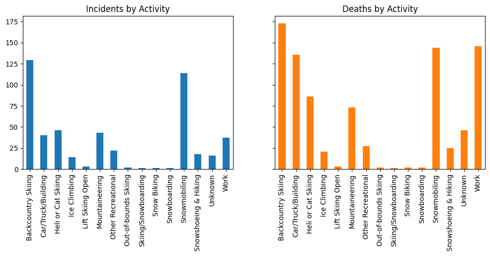
Now that we have incident data, let’s create some figures.

# clean up activity names
incidents.group_activity.unique()

array(['Skiing', 'Snowmobiling', 'Skiing/Snowboarding', 'Snow Biking',
       'Snowshoeing', 'Snowboarding', 'Backcountry Skiing',
       'Ice Climbing', 'Ski touring', 'Heliskiing',
       'Snowshoeing & Hiking', 'Mechanized Skiing', 'Work',
       'Mountaineering', 'Other Recreational', 'Out-of-bounds Skiing',
       'At Outdoor Worksite', 'Lift Skiing Closed', 'Lift Skiing Open',
       'Hunting/Fishing', 'Out-of-Bounds Skiing', 'Control Work',
       'Inside Building', 'Car/Truck on Road', 'Inside Car/Truck on Road',
       'Unknown', 'Outside Building'], dtype=object)

incidents.group_activity=incidents.group_activity.replace("Ski touring","Backcountry Skiing")
incidents.group_activity=incidents.group_activity.replace("Out-of-Bounds Skiing","Backcountry Skiing")
incidents.group_activity=incidents.group_activity.replace("Lift Skiing Closed","Backcountry Skiing")
incidents.group_activity=incidents.group_activity.replace("Skiing","Backcountry Skiing")
incidents.group_activity=incidents.group_activity.replace("Snowshoeing","Snowshoeing & Hiking")
incidents.group_activity=incidents.group_activity.replace("Snowshoeing and Hiking","Snowshoeing & Hiking")
incidents.group_activity=incidents.group_activity.replace("Mechanized Skiing","Heli or Cat Skiing")
incidents.group_activity=incidents.group_activity.replace("Heliskiing","Heli or Cat Skiing")
incidents.group_activity=incidents.group_activity.replace("At Outdoor Worksite","Work")
incidents.group_activity=incidents.group_activity.replace("Control Work","Work")
incidents.group_activity=incidents.group_activity.replace("Hunting/Fishing","Other Recreational")
incidents.group_activity=incidents.group_activity.replace("Inside Car/Truck on Road","Car/Truck/Building")
incidents.group_activity=incidents.group_activity.replace("Car/Truck on Road","Car/Truck/Building")
incidents.group_activity=incidents.group_activity.replace("Inside Building","Car/Truck/Building")
incidents.group_activity=incidents.group_activity.replace("Outside Building","Car/Truck/Building")


incidents.group_activity.unique()

fig, ax = plt.subplots(1,2, sharey=True, figsize=(12,4))
colors=plt.rcParams["axes.prop_cycle"].by_key()["color"]
incidents.groupby(['group_activity']).id.count().plot(kind='bar', title="Incidents by Activity", ax=ax[0])
incidents.groupby(['group_activity']).num_fatal.sum().plot(kind='bar', title="Deaths by Activity", ax=ax[1], color=colors[1])
ax[0].set_xlabel(None)
ax[1].set_xlabel(None);

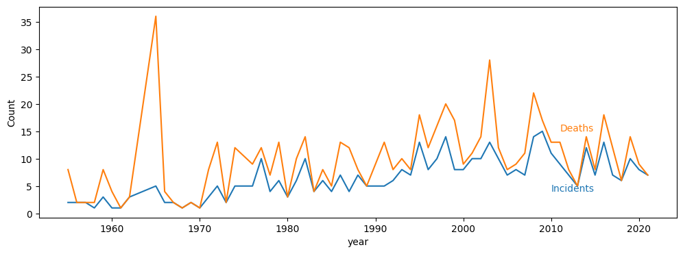
incidents["date"] = pd.to_datetime(incidents.ob_date)
incidents["year"] = incidents.date.apply(lambda x: x.year)
incidents.date = incidents.date.dt.date
colors=plt.rcParams["axes.prop_cycle"].by_key()["color"]
f = incidents.groupby(["year"]).num_fatal.sum()
n = incidents.groupby(["year"]).id.count()
yearstart=1950
f=f[f.index>yearstart]
n=n[n.index>yearstart]
fig,ax = plt.subplots(1,1,figsize=(12,4))
n.plot(ax=ax)
f.plot(ax=ax)
ax.set_ylabel("Count")
ax.annotate("Incidents", (2010, 4), color=colors[0])
ax.annotate("Deaths", (2011, 15), color=colors[1]);

Mapping Incidents

Since the incident data includes coordinates, we might as well make a map too. Unfortunately, some latitude and longitudes contain obvious errors. Here, we try to fix them.

import re

# fix errors in latitude, longitude
latlon = incidents.location_coords
def makenumeric(cstr):
    if cstr is None:
        return([None,None])
    elif (type(cstr)==str):
        return([float(s) for s in re.findall(r'-?\d+\.?\d*',cstr)])
    else:
        return(cstr)

latlon = latlon.apply(makenumeric)

def good_lat(lat):
    return(lat >= 41.6 and lat <= 83.12) # min & max for Canada

def good_lon(lon):
    return(lon >= -141 and lon<= -52.6)

def fixlatlon(c):
    if (len(c)<2 or type(c[0])!=float or type(c[1])!=float):
        c = [None, None]
        return(c)
    lat = c[0]
    lon = c[1]
    if not good_lat(lat) and good_lat(lon):
        tmp = lat
        lat = lon
        lon = tmp
    if not good_lon(lon) and good_lon(-lon):
        lon = -lon
    if not good_lon(lon) and good_lon(lat):
        tmp = lat
        lat = lon
        lon = tmp
    if not good_lon(lon) and good_lon(-lat):
        tmp = -lat
        lat = lon
        lon = tmp
    if not good_lat(lat) or not good_lon(lon):
        c[0] = None
        c[1] = None
    else:
        c[0] = lat
        c[1] = lon
    return(c)

incidents["latlon"] = latlon.apply(fixlatlon)

def foo(c, a):
    if (type(a)==str):
        a = [float(s) for s in re.findall(r'-?\d+\.?\d*',a)]
    if len(a) <2:
        a = [None,None]
    return([a[1],a[0]] if type(c[0])!=float else c)
incidents["latlon_filled"]=[foo(c,a) for c,a in zip(incidents["latlon"],incidents["alt_coord"])]
nmiss = sum([a[0]==None for a in incidents.latlon_filled])
n = len(incidents.latlon_filled)
print("{} of {} incidents have latitude & longitude".format(n-nmiss, n))

326 of 487 incidents have latitude & longitude

# download forecast region definitions
# req = urllib.request.Request("https://www.avalanche.ca/api/forecasts")
# The above link doesn't work since COVID-19 lockdown. Currently we use an old cached version instead
#req = ("https://web.archive.org/web/20150319031605if_/http://www.avalanche.ca/api/forecasts")
#with urllib.request.urlopen(req) as response:
#    forecastregions = json.loads(response.read().decode('utf-8'))
req = "https://faculty.arts.ubc.ca/pschrimpf/forecast-regions2015.json"
with urllib.request.urlopen(req) as response:
    regions2015 = json.loads(response.read().decode('utf-8'))

req = "https://faculty.arts.ubc.ca/pschrimpf/forecast-regions2019.json"
with urllib.request.urlopen(req) as response:
    regions2019 = json.loads(response.read().decode('utf-8'))

forecastregions = regions2019
ids = [r['id'] for r in forecastregions['features']]
for r in regions2015['features'] :
     if not r['id'] in ids :
            forecastregions['features'].append(r)

You may have to uncomment the second line below if folium is not installed.

# Map forecast regions and incidents
#!pip install --user folium
import folium
import matplotlib

cmap = matplotlib.colormaps["Set1"]
fmap = folium.Map(location=[60, -98],
                            zoom_start=3)
with urllib.request.urlopen(req) as response:
    regions_tmp = json.loads(response.read().decode('utf-8'))
folium.GeoJson(regions_tmp,
               tooltip=folium.GeoJsonTooltip(fields=["name"], aliases=[""]),
               highlight_function=lambda x: { 'weight': 10},
              style_function=lambda x: {'weight':1}).add_to(fmap)
activities = incidents.group_activity.unique()
for i in incidents.index:
    if incidents.latlon_filled[i][0] is not None and  incidents.latlon_filled[i][1] is not None:
        cindex=[j for j,x in enumerate(activities) if x==incidents.group_activity[i]][0]
        txt = "{}, {}<br>{} deaths"
        txt = txt.format(incidents.group_activity[i],
                        incidents.ob_date[i],
                        incidents.num_fatal[i]
                        )
        pop = folium.Popup(incidents.comment[i], parse_html=True, max_width=400)
        folium.CircleMarker(incidents.latlon_filled[i],
                      tooltip=txt,
                      popup=pop,
                      color=matplotlib.colors.to_hex(cmap(cindex)), fill=True, radius=5).add_to(fmap)
fmap

Make this Notebook Trusted to load map: File -> Trust Notebook

Take a moment to click around the map and read about some of the incidents.

Between presenting this information on a map and the list on https://www.avalanche.ca/incidents/ , which do you prefer and why?

Matching Incidents to Regions

Later, we will want to match incidents to forecasts, so let’s find the closest region to each incident.

Note that distance here will be in units of latitude, longitude (or whatever coordinate system we use). At the equator, a distance of 1 is approximately 60 nautical miles.

Since longitude lines get closer together farther from the equator, these distances will be understated the further North you go.

This is not much of a problem if we’re just finding the nearest region, but if we care about accurate distances, we should re-project the latitude and longitude into a different coordinate system.

# Match incidents to nearest forecast regions.
from shapely.geometry import Point, Polygon, shape
point = Point(incidents.latlon_filled[0][1],incidents.latlon_filled[0][0])
def distances(latlon):
    point=Point(latlon[1],latlon[0])
    df = pd.DataFrame.from_dict([{'id':feature['id'],
                                  'distance':shape(feature['geometry']).distance(point)} for
                                 feature in forecastregions['features']])
    return(df)
def foo(x):
    if (x[0]==None):
        return(None)
    d = distances(x)
    return(d.id[d.distance.idxmin()])
incidents['nearest_region'] = incidents.latlon_filled.apply(foo)
incidents['nearest_distance'] = incidents.latlon_filled.apply(lambda x: None if x[0]==None else distances(x).distance.min())

incidents

	Unnamed: 0	id	ob_date	location	...	latlon	latlon_filled	nearest_region	nearest_distance
0	0	ba14a125-29f7-4432-97ad-73a53207a5e7	2021-04-05	Haddo Peak	...	[51.38329, -116.23453]	[51.38329, -116.23453]	banff-yoho-kootenay	0.000000
1	1	59023c05-b679-4e9f-9c06-910021318663	2021-03-29	Eureka Peak	...	[52.33517, -120.69033]	[52.33517, -120.69033]	cariboos	0.000000
2	2	10774b2d-b7de-42ac-a600-9828cb4e6129	2021-03-04	Reco Mountain	...	[49.99979, -117.18904]	[49.99979, -117.18904]	south-columbia	0.000000
3	3	4f79d4db-57b3-4843-909f-eaca3c499e7c	2021-02-23	Swift Creek	...	[52.917303, -119.081732]	[52.917303, -119.081732]	north-rockies	0.086401
4	4	a6115fd5-b330-4424-b400-4bc218f387e1	2021-02-20	Hasler	...	[55.3377373, -122.256577]	[55.3377373, -122.256577]	north-rockies	0.000000
...	...	...	...	...	...	...	...	...	...
482	482	101c517b-29a4-4c49-8934-f6c56ddd882d	1840-02-01	Château-Richer	...	[None, None]	[46.9666667, -71.0166667]	chic-chocs	5.145266
483	483	b2e1c50a-1533-4145-a1a2-0befca0154d5	1836-02-09	Quebec	...	[None, None]	[46.813819, -71.207997]	chic-chocs	5.380364
484	484	18e8f963-da33-4682-9312-57ca2cc9ad8d	1833-05-24	Carbonear	...	[47.733333587646484, -53.21666717529297]	[47.733333587646484, -53.21666717529297]	chic-chocs	12.827272
485	485	083d22df-ed50-4687-b9ab-1649960a0fbe	1825-02-04	Saint-Joseph de Lévis	...	[None, None]	[46.8105556, -71.1819444]	chic-chocs	5.357613
486	486	f498c48a-981d-43cf-ac16-151b8794435c	1782-01-01	Nain	...	[56.53333282470703, -61.68333435058594]	[56.53333282470703, -61.68333435058594]	chic-chocs	8.633647

487 rows × 27 columns

Forecast Data

We’ll now download all forecasts for all regions since November 2011 (roughly the earliest data available).

We can only request one forecast at a time, so this takes many hours to download.

To make this process run more quickly for readers, we ran the code ourselves and then stored the data in the cloud.

The function below will fetch all the forecasts from the cloud storage location and save them to a folder named avalanche_forecasts.

def download_cached_forecasts():
    # download the zipped file and unzip it here
    url = "https://datascience.quantecon.org/assets/data/avalanche_forecasts.zip?raw=true"
    with requests.get(url) as res:
        if not res.ok:
            raise ValueError("failed to download the cached forecasts")
        with zipfile.ZipFile(io.BytesIO(res.content)) as z:
            for f in z.namelist():
                if (os.path.isfile(f) and z.getinfo(f).file_size < os.stat(f).st_size):
                    warnings.warn(f"'File $f exists and is larger than version in cache. Not replacing.")
                else :
                    z.extract(f)
                    print("Downloaded and extracted", f)

download_cached_forecasts()

Downloaded and extracted avalanche_forecasts/banff-yoho-kootenay_2011-2012.json
Downloaded and extracted avalanche_forecasts/banff-yoho-kootenay_2012-2013.json
Downloaded and extracted avalanche_forecasts/banff-yoho-kootenay_2013-2014.json
Downloaded and extracted avalanche_forecasts/banff-yoho-kootenay_2014-2015.json
Downloaded and extracted avalanche_forecasts/banff-yoho-kootenay_2015-2016.json
Downloaded and extracted avalanche_forecasts/banff-yoho-kootenay_2016-2017.json
Downloaded and extracted avalanche_forecasts/banff-yoho-kootenay_2017-2018.json
Downloaded and extracted avalanche_forecasts/banff-yoho-kootenay_2018-2019.json
Downloaded and extracted avalanche_forecasts/cariboos_2011-2012.json
Downloaded and extracted avalanche_forecasts/cariboos_2012-2013.json
Downloaded and extracted avalanche_forecasts/cariboos_2013-2014.json
Downloaded and extracted avalanche_forecasts/cariboos_2014-2015.json
Downloaded and extracted avalanche_forecasts/cariboos_2015-2016.json
Downloaded and extracted avalanche_forecasts/cariboos_2016-2017.json
Downloaded and extracted avalanche_forecasts/cariboos_2017-2018.json
Downloaded and extracted avalanche_forecasts/cariboos_2018-2019.json
Downloaded and extracted avalanche_forecasts/chic-chocs_2011-2012.json
Downloaded and extracted avalanche_forecasts/chic-chocs_2012-2013.json
Downloaded and extracted avalanche_forecasts/chic-chocs_2013-2014.json
Downloaded and extracted avalanche_forecasts/chic-chocs_2014-2015.json
Downloaded and extracted avalanche_forecasts/chic-chocs_2015-2016.json
Downloaded and extracted avalanche_forecasts/chic-chocs_2016-2017.json
Downloaded and extracted avalanche_forecasts/chic-chocs_2017-2018.json
Downloaded and extracted avalanche_forecasts/chic-chocs_2018-2019.json
Downloaded and extracted avalanche_forecasts/glacier_2011-2012.json
Downloaded and extracted avalanche_forecasts/glacier_2012-2013.json
Downloaded and extracted avalanche_forecasts/glacier_2013-2014.json
Downloaded and extracted avalanche_forecasts/glacier_2014-2015.json
Downloaded and extracted avalanche_forecasts/glacier_2015-2016.json
Downloaded and extracted avalanche_forecasts/glacier_2016-2017.json
Downloaded and extracted avalanche_forecasts/glacier_2017-2018.json
Downloaded and extracted avalanche_forecasts/glacier_2018-2019.json
Downloaded and extracted avalanche_forecasts/hankin-evelyn_2011-2012.json
Downloaded and extracted avalanche_forecasts/hankin-evelyn_2012-2013.json
Downloaded and extracted avalanche_forecasts/hankin-evelyn_2013-2014.json
Downloaded and extracted avalanche_forecasts/hankin-evelyn_2014-2015.json
Downloaded and extracted avalanche_forecasts/hankin-evelyn_2015-2016.json
Downloaded and extracted avalanche_forecasts/hankin-evelyn_2016-2017.json
Downloaded and extracted avalanche_forecasts/hankin-evelyn_2017-2018.json
Downloaded and extracted avalanche_forecasts/hankin-evelyn_2018-2019.json
Downloaded and extracted avalanche_forecasts/jasper_2011-2012.json
Downloaded and extracted avalanche_forecasts/jasper_2012-2013.json
Downloaded and extracted avalanche_forecasts/jasper_2013-2014.json
Downloaded and extracted avalanche_forecasts/jasper_2014-2015.json
Downloaded and extracted avalanche_forecasts/jasper_2015-2016.json
Downloaded and extracted avalanche_forecasts/jasper_2016-2017.json
Downloaded and extracted avalanche_forecasts/jasper_2017-2018.json
Downloaded and extracted avalanche_forecasts/jasper_2018-2019.json
Downloaded and extracted avalanche_forecasts/kakwa_2011-2012.json
Downloaded and extracted avalanche_forecasts/kakwa_2012-2013.json
Downloaded and extracted avalanche_forecasts/kakwa_2013-2014.json
Downloaded and extracted avalanche_forecasts/kakwa_2014-2015.json
Downloaded and extracted avalanche_forecasts/kakwa_2015-2016.json
Downloaded and extracted avalanche_forecasts/kakwa_2016-2017.json
Downloaded and extracted avalanche_forecasts/kakwa_2017-2018.json
Downloaded and extracted avalanche_forecasts/kakwa_2018-2019.json
Downloaded and extracted avalanche_forecasts/kananaskis_2011-2012.json
Downloaded and extracted avalanche_forecasts/kananaskis_2012-2013.json
Downloaded and extracted avalanche_forecasts/kananaskis_2013-2014.json
Downloaded and extracted avalanche_forecasts/kananaskis_2014-2015.json
Downloaded and extracted avalanche_forecasts/kananaskis_2015-2016.json
Downloaded and extracted avalanche_forecasts/kananaskis_2016-2017.json
Downloaded and extracted avalanche_forecasts/kananaskis_2017-2018.json
Downloaded and extracted avalanche_forecasts/kananaskis_2018-2019.json
Downloaded and extracted avalanche_forecasts/kootenay-boundary_2011-2012.json
Downloaded and extracted avalanche_forecasts/kootenay-boundary_2012-2013.json
Downloaded and extracted avalanche_forecasts/kootenay-boundary_2013-2014.json
Downloaded and extracted avalanche_forecasts/kootenay-boundary_2014-2015.json
Downloaded and extracted avalanche_forecasts/kootenay-boundary_2015-2016.json
Downloaded and extracted avalanche_forecasts/kootenay-boundary_2016-2017.json
Downloaded and extracted avalanche_forecasts/kootenay-boundary_2017-2018.json
Downloaded and extracted avalanche_forecasts/kootenay-boundary_2018-2019.json
Downloaded and extracted avalanche_forecasts/little-yoho_2011-2012.json
Downloaded and extracted avalanche_forecasts/little-yoho_2012-2013.json
Downloaded and extracted avalanche_forecasts/little-yoho_2013-2014.json
Downloaded and extracted avalanche_forecasts/little-yoho_2014-2015.json
Downloaded and extracted avalanche_forecasts/little-yoho_2015-2016.json
Downloaded and extracted avalanche_forecasts/little-yoho_2016-2017.json
Downloaded and extracted avalanche_forecasts/little-yoho_2017-2018.json
Downloaded and extracted avalanche_forecasts/little-yoho_2018-2019.json
Downloaded and extracted avalanche_forecasts/lizard-range_2011-2012.json
Downloaded and extracted avalanche_forecasts/lizard-range_2012-2013.json
Downloaded and extracted avalanche_forecasts/lizard-range_2013-2014.json
Downloaded and extracted avalanche_forecasts/lizard-range_2014-2015.json
Downloaded and extracted avalanche_forecasts/lizard-range_2015-2016.json
Downloaded and extracted avalanche_forecasts/lizard-range_2016-2017.json
Downloaded and extracted avalanche_forecasts/lizard-range_2017-2018.json
Downloaded and extracted avalanche_forecasts/lizard-range_2018-2019.json
Downloaded and extracted avalanche_forecasts/north-columbia_2011-2012.json
Downloaded and extracted avalanche_forecasts/north-columbia_2012-2013.json
Downloaded and extracted avalanche_forecasts/north-columbia_2013-2014.json
Downloaded and extracted avalanche_forecasts/north-columbia_2014-2015.json
Downloaded and extracted avalanche_forecasts/north-columbia_2015-2016.json
Downloaded and extracted avalanche_forecasts/north-columbia_2016-2017.json
Downloaded and extracted avalanche_forecasts/north-columbia_2017-2018.json
Downloaded and extracted avalanche_forecasts/north-columbia_2018-2019.json
Downloaded and extracted avalanche_forecasts/north-rockies_2011-2012.json
Downloaded and extracted avalanche_forecasts/north-rockies_2012-2013.json
Downloaded and extracted avalanche_forecasts/north-rockies_2013-2014.json
Downloaded and extracted avalanche_forecasts/north-rockies_2014-2015.json
Downloaded and extracted avalanche_forecasts/north-rockies_2015-2016.json
Downloaded and extracted avalanche_forecasts/north-rockies_2016-2017.json
Downloaded and extracted avalanche_forecasts/north-rockies_2017-2018.json
Downloaded and extracted avalanche_forecasts/north-rockies_2018-2019.json
Downloaded and extracted avalanche_forecasts/north-shore_2011-2012.json
Downloaded and extracted avalanche_forecasts/north-shore_2012-2013.json
Downloaded and extracted avalanche_forecasts/north-shore_2013-2014.json
Downloaded and extracted avalanche_forecasts/north-shore_2014-2015.json
Downloaded and extracted avalanche_forecasts/north-shore_2015-2016.json
Downloaded and extracted avalanche_forecasts/north-shore_2016-2017.json
Downloaded and extracted avalanche_forecasts/north-shore_2017-2018.json
Downloaded and extracted avalanche_forecasts/north-shore_2018-2019.json
Downloaded and extracted avalanche_forecasts/northwest-coastal_2011-2012.json
Downloaded and extracted avalanche_forecasts/northwest-coastal_2012-2013.json
Downloaded and extracted avalanche_forecasts/northwest-coastal_2013-2014.json
Downloaded and extracted avalanche_forecasts/northwest-coastal_2014-2015.json
Downloaded and extracted avalanche_forecasts/northwest-coastal_2015-2016.json
Downloaded and extracted avalanche_forecasts/northwest-coastal_2016-2017.json
Downloaded and extracted avalanche_forecasts/northwest-coastal_2017-2018.json
Downloaded and extracted avalanche_forecasts/northwest-coastal_2018-2019.json
Downloaded and extracted avalanche_forecasts/northwest-inland_2011-2012.json
Downloaded and extracted avalanche_forecasts/northwest-inland_2012-2013.json
Downloaded and extracted avalanche_forecasts/northwest-inland_2013-2014.json
Downloaded and extracted avalanche_forecasts/northwest-inland_2014-2015.json
Downloaded and extracted avalanche_forecasts/northwest-inland_2015-2016.json
Downloaded and extracted avalanche_forecasts/northwest-inland_2016-2017.json
Downloaded and extracted avalanche_forecasts/northwest-inland_2017-2018.json
Downloaded and extracted avalanche_forecasts/northwest-inland_2018-2019.json
Downloaded and extracted avalanche_forecasts/purcells_2011-2012.json
Downloaded and extracted avalanche_forecasts/purcells_2012-2013.json
Downloaded and extracted avalanche_forecasts/purcells_2013-2014.json
Downloaded and extracted avalanche_forecasts/purcells_2014-2015.json
Downloaded and extracted avalanche_forecasts/purcells_2015-2016.json
Downloaded and extracted avalanche_forecasts/purcells_2016-2017.json
Downloaded and extracted avalanche_forecasts/purcells_2017-2018.json
Downloaded and extracted avalanche_forecasts/purcells_2018-2019.json
Downloaded and extracted avalanche_forecasts/renshaw_2011-2012.json
Downloaded and extracted avalanche_forecasts/renshaw_2012-2013.json
Downloaded and extracted avalanche_forecasts/renshaw_2013-2014.json
Downloaded and extracted avalanche_forecasts/renshaw_2014-2015.json
Downloaded and extracted avalanche_forecasts/renshaw_2015-2016.json
Downloaded and extracted avalanche_forecasts/renshaw_2016-2017.json
Downloaded and extracted avalanche_forecasts/renshaw_2017-2018.json
Downloaded and extracted avalanche_forecasts/renshaw_2018-2019.json
Downloaded and extracted avalanche_forecasts/sea-to-sky_2011-2012.json
Downloaded and extracted avalanche_forecasts/sea-to-sky_2012-2013.json
Downloaded and extracted avalanche_forecasts/sea-to-sky_2013-2014.json
Downloaded and extracted avalanche_forecasts/sea-to-sky_2014-2015.json
Downloaded and extracted avalanche_forecasts/sea-to-sky_2015-2016.json
Downloaded and extracted avalanche_forecasts/sea-to-sky_2016-2017.json
Downloaded and extracted avalanche_forecasts/sea-to-sky_2017-2018.json
Downloaded and extracted avalanche_forecasts/sea-to-sky_2018-2019.json
Downloaded and extracted avalanche_forecasts/south-coast_2011-2012.json
Downloaded and extracted avalanche_forecasts/south-coast_2012-2013.json
Downloaded and extracted avalanche_forecasts/south-coast_2013-2014.json
Downloaded and extracted avalanche_forecasts/south-coast_2014-2015.json
Downloaded and extracted avalanche_forecasts/south-coast_2015-2016.json
Downloaded and extracted avalanche_forecasts/south-coast_2016-2017.json
Downloaded and extracted avalanche_forecasts/south-coast_2017-2018.json
Downloaded and extracted avalanche_forecasts/south-coast_2018-2019.json
Downloaded and extracted avalanche_forecasts/south-coast-inland_2011-2012.json
Downloaded and extracted avalanche_forecasts/south-coast-inland_2012-2013.json
Downloaded and extracted avalanche_forecasts/south-coast-inland_2013-2014.json
Downloaded and extracted avalanche_forecasts/south-coast-inland_2014-2015.json
Downloaded and extracted avalanche_forecasts/south-coast-inland_2015-2016.json
Downloaded and extracted avalanche_forecasts/south-coast-inland_2016-2017.json
Downloaded and extracted avalanche_forecasts/south-coast-inland_2017-2018.json
Downloaded and extracted avalanche_forecasts/south-coast-inland_2018-2019.json
Downloaded and extracted avalanche_forecasts/south-columbia_2011-2012.json
Downloaded and extracted avalanche_forecasts/south-columbia_2012-2013.json
Downloaded and extracted avalanche_forecasts/south-columbia_2013-2014.json
Downloaded and extracted avalanche_forecasts/south-columbia_2014-2015.json
Downloaded and extracted avalanche_forecasts/south-columbia_2015-2016.json
Downloaded and extracted avalanche_forecasts/south-columbia_2016-2017.json
Downloaded and extracted avalanche_forecasts/south-columbia_2017-2018.json
Downloaded and extracted avalanche_forecasts/south-columbia_2018-2019.json
Downloaded and extracted avalanche_forecasts/south-rockies_2011-2012.json
Downloaded and extracted avalanche_forecasts/south-rockies_2012-2013.json
Downloaded and extracted avalanche_forecasts/south-rockies_2013-2014.json
Downloaded and extracted avalanche_forecasts/south-rockies_2014-2015.json
Downloaded and extracted avalanche_forecasts/south-rockies_2015-2016.json
Downloaded and extracted avalanche_forecasts/south-rockies_2016-2017.json
Downloaded and extracted avalanche_forecasts/south-rockies_2017-2018.json
Downloaded and extracted avalanche_forecasts/south-rockies_2018-2019.json
Downloaded and extracted avalanche_forecasts/telkwa_2011-2012.json
Downloaded and extracted avalanche_forecasts/telkwa_2012-2013.json
Downloaded and extracted avalanche_forecasts/telkwa_2013-2014.json
Downloaded and extracted avalanche_forecasts/telkwa_2014-2015.json
Downloaded and extracted avalanche_forecasts/telkwa_2015-2016.json
Downloaded and extracted avalanche_forecasts/telkwa_2016-2017.json
Downloaded and extracted avalanche_forecasts/telkwa_2017-2018.json
Downloaded and extracted avalanche_forecasts/telkwa_2018-2019.json
Downloaded and extracted avalanche_forecasts/vancouver-island_2011-2012.json
Downloaded and extracted avalanche_forecasts/vancouver-island_2012-2013.json
Downloaded and extracted avalanche_forecasts/vancouver-island_2013-2014.json
Downloaded and extracted avalanche_forecasts/vancouver-island_2014-2015.json
Downloaded and extracted avalanche_forecasts/vancouver-island_2015-2016.json
Downloaded and extracted avalanche_forecasts/vancouver-island_2016-2017.json
Downloaded and extracted avalanche_forecasts/vancouver-island_2017-2018.json
Downloaded and extracted avalanche_forecasts/vancouver-island_2018-2019.json
Downloaded and extracted avalanche_forecasts/waterton_2011-2012.json
Downloaded and extracted avalanche_forecasts/waterton_2012-2013.json
Downloaded and extracted avalanche_forecasts/waterton_2013-2014.json
Downloaded and extracted avalanche_forecasts/waterton_2014-2015.json
Downloaded and extracted avalanche_forecasts/waterton_2015-2016.json
Downloaded and extracted avalanche_forecasts/waterton_2016-2017.json
Downloaded and extracted avalanche_forecasts/waterton_2017-2018.json
Downloaded and extracted avalanche_forecasts/waterton_2018-2019.json
Downloaded and extracted avalanche_forecasts/whistler-blackcomb_2011-2012.json
Downloaded and extracted avalanche_forecasts/whistler-blackcomb_2012-2013.json
Downloaded and extracted avalanche_forecasts/whistler-blackcomb_2013-2014.json
Downloaded and extracted avalanche_forecasts/whistler-blackcomb_2014-2015.json
Downloaded and extracted avalanche_forecasts/whistler-blackcomb_2015-2016.json
Downloaded and extracted avalanche_forecasts/whistler-blackcomb_2016-2017.json
Downloaded and extracted avalanche_forecasts/whistler-blackcomb_2017-2018.json
Downloaded and extracted avalanche_forecasts/whistler-blackcomb_2018-2019.json
Downloaded and extracted avalanche_forecasts/yukon_2011-2012.json
Downloaded and extracted avalanche_forecasts/yukon_2012-2013.json
Downloaded and extracted avalanche_forecasts/yukon_2013-2014.json
Downloaded and extracted avalanche_forecasts/yukon_2014-2015.json
Downloaded and extracted avalanche_forecasts/yukon_2015-2016.json
Downloaded and extracted avalanche_forecasts/yukon_2016-2017.json
Downloaded and extracted avalanche_forecasts/yukon_2017-2018.json
Downloaded and extracted avalanche_forecasts/yukon_2018-2019.json

The code below is what we initially ran to obtain all the forecasts.

You will notice that this code checks to see whether the files can be found in the avalanche_forecasts directory (they can if you ran the download_cached_forecasts above!) and will only download them if they aren’t found.

You can experiment with this caching by deleting one or more files from the avalanche_forecasts folder and re-running the cells below.

# Functions for downloading forecasts from Avalanche Canada

def get_forecast(date, region):
    url = "https://www.avalanche.ca/api/bulletin-archive/{}/{}.json".format(date.isoformat(),region)
    try:
        req = urllib.request.Request(url)
        with urllib.request.urlopen(req) as response:
            result = json.loads(response.read().decode('utf-8'))
        return(result)
    except:
        return(None)

def get_forecasts(start, end, region):
    day = start
    forecasts = []
    while(day<=end and day<end.today()):
        #print("working on {}, {}".format(region,day))
        forecasts = forecasts + [get_forecast(day, region)]
        #print("sleeping")
        time.sleep(0.01) # to avoid too much load on Avalanche Canada servers
        day = day + pd.Timedelta(1,"D")
    return(forecasts)

def get_season(year, region):
    start_month = 11
    start_day = 20
    last_month = 5
    last_day = 1
    if (not os.path.isdir("avalanche_forecasts")):
        os.mkdir("avalanche_forecasts")
    seasonfile = "avalanche_forecasts/{}_{}-{}.json".format(region, year, year+1)
    if (not os.path.isfile(seasonfile)):
        print(f"Season file {seasonfile} not found. Uncomment code here to update cached data")
        season = []
        #startdate = pd.to_datetime("{}-{}-{} 12:00".format(year, start_month, start_day))
        #lastdate = pd.to_datetime("{}-{}-{} 12:00".format(year+1, last_month, last_day))
        #season = get_forecasts(startdate,lastdate,region)
        #with open(seasonfile, 'w') as outfile:
        #    json.dump(season, outfile, ensure_ascii=False)
    else:
        with open(seasonfile, "rb") as json_data:
            season = json.load(json_data)
    return(season)

forecastlist=[]

for year in range(2011,2019):
    print("working on {}".format(year))
    for region in [region["id"] for region in forecastregions["features"]]:
        forecastlist = forecastlist + get_season(year, region)

working on 2011
working on 2012
working on 2013

working on 2014
working on 2015
working on 2016
working on 2017

working on 2018

# convert to DataFrame and extract some variables
forecasts = pd.DataFrame.from_dict([f for f in forecastlist if not f==None],orient="columns")

forecasts["danger_date"] = forecasts.dangerRatings.apply(lambda r: r[0]["date"])
forecasts["danger_date"] = pd.to_datetime(forecasts.danger_date, format='ISO8601').dt.date
forecasts["danger_alpine"]=forecasts.dangerRatings.apply(lambda r: r[0]["dangerRating"]["alp"])
forecasts["danger_treeline"]=forecasts.dangerRatings.apply(lambda r: r[0]["dangerRating"]["tln"])
forecasts["danger_belowtree"]=forecasts.dangerRatings.apply(lambda r: r[0]["dangerRating"]["btl"])

forecasts.head()

	id	region	dateIssued	validUntil	...	danger_date	danger_alpine	danger_treeline	danger_belowtree
0	bid_29924	northwest-coastal	2011-11-20T00:49:00.000Z	2011-11-21T00:00:00.000Z	...	2011-11-21	2:Moderate	2:Moderate	1:Low
1	bid_29943	northwest-coastal	2011-11-21T01:00:00.000Z	2011-11-22T00:00:00.000Z	...	2011-11-22	3:Considerable	3:Considerable	2:Moderate
2	bid_29965	northwest-coastal	2011-11-22T01:43:00.000Z	2011-11-23T00:00:00.000Z	...	2011-11-23	4:High	4:High	3:Considerable
3	bid_30080	northwest-coastal	2011-11-23T01:38:00.000Z	2011-11-24T00:00:00.000Z	...	2011-11-24	4:High	4:High	3:Considerable
4	bid_30358	northwest-coastal	2011-11-24T00:55:00.000Z	2011-11-25T00:00:00.000Z	...	2011-11-25	4:High	4:High	3:Considerable

5 rows × 18 columns

# merge incidents to forecasts
adf = pd.merge(forecasts, incidents, how="left",
               left_on=["region","danger_date"],
               right_on=["nearest_region","date"],
              indicator=True)
adf["incident"] = adf._merge=="both"
print("There were {} incidents matched with forecasts data. These occured on {}% of day-regions with forecasts".format(adf.incident.sum(),adf.incident.mean()*100))

There were 39 incidents matched with forecasts data. These occured on 0.26666666666666666% of day-regions with forecasts

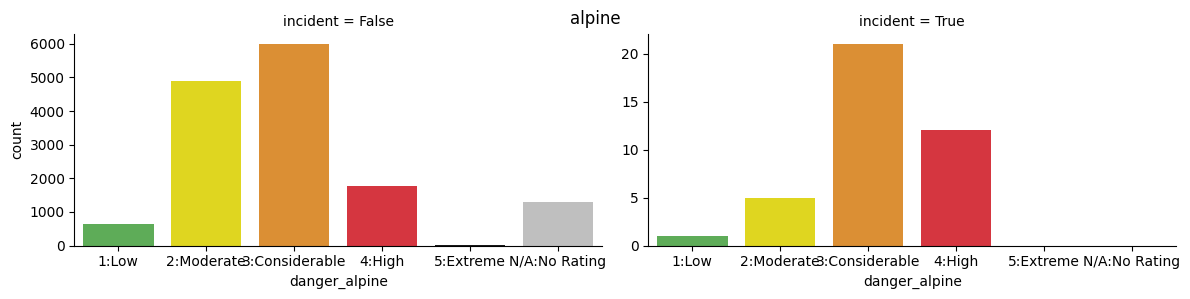
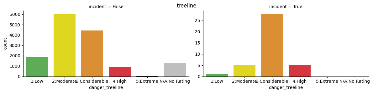
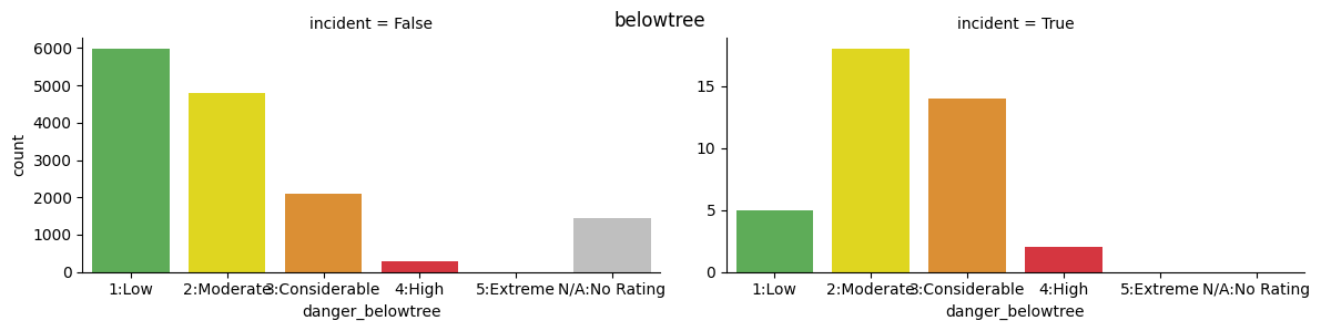
import seaborn as sns
ratings=sorted(adf.danger_alpine.unique())
ava_colors = ["#52BA4A", "#FFF300", "#F79218", "#EF1C29", "#1A1A1A", "#BFBFBF"]
for x in ["danger_alpine", "danger_treeline", "danger_belowtree"]:
    fig=sns.catplot(x=x, kind="count",col="incident", order=ratings, data=adf, sharey=False,
                    palette=ava_colors, height=3, aspect=2)
    plt.subplots_adjust(top=0.9)
    fig.fig.suptitle(x.replace("danger_",""))
    display(fig)

/tmp/ipykernel_2801/2760332395.py:5: FutureWarning: 

Passing `palette` without assigning `hue` is deprecated and will be removed in v0.14.0. Assign the `x` variable to `hue` and set `legend=False` for the same effect.

  fig=sns.catplot(x=x, kind="count",col="incident", order=ratings, data=adf, sharey=False,

<seaborn.axisgrid.FacetGrid at 0x7ff048f64b90>

/tmp/ipykernel_2801/2760332395.py:5: FutureWarning: 

Passing `palette` without assigning `hue` is deprecated and will be removed in v0.14.0. Assign the `x` variable to `hue` and set `legend=False` for the same effect.

  fig=sns.catplot(x=x, kind="count",col="incident", order=ratings, data=adf, sharey=False,

<seaborn.axisgrid.FacetGrid at 0x7ff047a784d0>

/tmp/ipykernel_2801/2760332395.py:5: FutureWarning: 

Passing `palette` without assigning `hue` is deprecated and will be removed in v0.14.0. Assign the `x` variable to `hue` and set `legend=False` for the same effect.

  fig=sns.catplot(x=x, kind="count",col="incident", order=ratings, data=adf, sharey=False,

<seaborn.axisgrid.FacetGrid at 0x7ff047b170b0>

Predicting Incidents from Text

Preprocessing

The first step when using text as data is to pre-process the text.

In preprocessing, we will:

1. Clean: Remove unwanted punctuation and non-text characters.

2. Tokenize: Break sentences down into words.

3. Remove “stopwords”: Eliminate common words that actually provide no information, like “a” and “the”.

4. Lemmatize words: Reduce words to their dictionary “lemma” e.g. “snowing” and “snowed” both become snow (verb).

from bs4 import BeautifulSoup
import nltk
import string
nltk.download('omw-1.4')
nltk.download('punkt')
nltk.download('punkt_tab')
nltk.download('stopwords')
nltk.download('wordnet')
# Remove stopwords (the, a, is, etc)
stopwords = set(nltk.corpus.stopwords.words('english'))
stopwords=stopwords.union(set(string.punctuation))
# Lemmatize words e.g. snowed and snowing are both snow (verb)
wnl = nltk.WordNetLemmatizer()
def text_prep(txt):
    soup = BeautifulSoup(txt, "lxml")
    [s.extract() for s in soup('style')] # remove css
    txt=soup.text # remove html tags
    txt = txt.lower()
    tokens = [token for token in nltk.tokenize.word_tokenize(txt)]
    tokens = [token for token in tokens if not token in stopwords]
    #tokens = [token for token in tokens if not token ]
    tokens = [wnl.lemmatize(token) for token in tokens]
    if (len(tokens)==0):
        tokens = ["EMPTYSTRING"]
    return(tokens)

text_prep(forecasts.highlights[1000])

[nltk_data] Downloading package omw-1.4 to /home/runner/nltk_data...

[nltk_data] Downloading package punkt to /home/runner/nltk_data...
[nltk_data]   Unzipping tokenizers/punkt.zip.

[nltk_data] Downloading package punkt_tab to /home/runner/nltk_data...
[nltk_data]   Unzipping tokenizers/punkt_tab.zip.
[nltk_data] Downloading package stopwords to /home/runner/nltk_data...
[nltk_data]   Unzipping corpora/stopwords.zip.
[nltk_data] Downloading package wordnet to /home/runner/nltk_data...

['avalanche',
 'danger',
 'could',
 'spike',
 'high',
 'slope',
 'getting',
 'baked',
 'sun',
 'avoid',
 'traveling',
 'underneath',
 'area']

Now, let’s apply this to all avalanche summaries.

text_data = [text_prep(txt) for txt in adf.avalancheSummary]

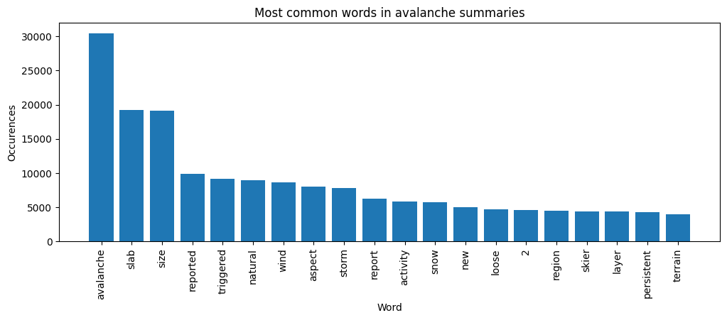
Let’s make a bar plot of the most common words.

wf = nltk.FreqDist([word for doc in text_data for word in doc]).most_common(20)
words = [x[0] for x in wf]
cnt = [x[1] for x in wf]

fig, ax = plt.subplots(figsize=(12,4))
ax.bar(range(len(words)), cnt);
ax.set_xticks(range(len(words)));
ax.set_xticklabels(words, rotation='vertical');
ax.set_title('Most common words in avalanche summaries');
ax.set_xlabel('Word');
ax.set_ylabel('Occurences');
plt.show()

Feature Engineering

The “bag of words” approach is the simplest way to convert a collection of processed text documents to a feature matrix. We view each document as a bag of words, and our feature matrix counts how many times each word appears. This method is called a “bag of words” because we ignore the document’s word order.

from sklearn.feature_extraction.text import CountVectorizer, TfidfVectorizer
vectorizer = CountVectorizer(max_features=500, min_df=5, max_df=0.7)
text_data = [text_prep(txt) for txt in adf.avalancheSummary]
y = adf.incident
X = vectorizer.fit_transform([' '.join(doc) for doc in text_data])

We can also perform more complicated feature engineering. One extension of the “bag of words” method is to consider counts of pairs or triples of consecutive words. These are called n-grams and can be created by setting the n_gram argument to CountVectorizer. Another alternative might be to accommodate the fact that common words will inherently have higher counts by using term-frequency inverse-document-frequency (see below).

After creating our feature matrix, we can now apply any classification method to predict incidents.

Naive Bayes Classifier

A common text data classifier is the Naive Bayes classifier. This classifier predicts incidents using Bayes’ rules.

\[ P(incident | words) = \frac{P(words|incident) P(incidents)}{P(words)} \]

The classifier is naive, though; it assumes words are independent of one another in any given incident.

\[ P(words|incident) = \prod_{w \in words} P(w|incident) \]

Although this assumption is implausible for text, the Naive Bayes classifier can be computed extremely quickly, and sometimes quite well.

from sklearn.model_selection import train_test_split
Xtrain, Xtest, ytrain, ytest = train_test_split(X, y, test_size=0.3, random_state=124)

from sklearn import naive_bayes
classifier = naive_bayes.MultinomialNB()
classifier.fit(Xtrain,ytrain)
np.mean(classifier.predict(Xtest)==ytest)

0.9933910665451231

from sklearn import metrics
print(metrics.confusion_matrix(ytest, classifier.predict(Xtest)))
print(metrics.classification_report(ytest, classifier.predict(Xtest)))

[[4358   18]
 [  11    1]]
              precision    recall  f1-score   support

       False       1.00      1.00      1.00      4376
        True       0.05      0.08      0.06        12

    accuracy                           0.99      4388
   macro avg       0.53      0.54      0.53      4388
weighted avg       0.99      0.99      0.99      4388

# print text with highest predicted probabilities
phat=classifier.predict_proba(X)[:,1]
def remove_html(txt):
    soup = BeautifulSoup(txt, "lxml")
    [s.extract() for s in soup('style')] # remove css
    return(soup.text)
docs = [remove_html(txt) for txt in adf.avalancheSummary]
txt_high = [(_,x) for _, x in sorted(zip(phat,docs), key=lambda pair: pair[0],reverse=True)]
txt_high[:10]

[(0.9993519607652722,
  "In the dogtooth backcountry, observers reported a size 2.5 avalanche with a crown 1m+ in depth, that was likely human triggered.  Remote triggering of avalanches continues to be reported from the region.  Explosive control work once again produced large avalanches to size 3.5 on all aspects with crowns ranging from 40 - 120 in depth.I've left the previous narratives in from earlier this because they help to illustrate the nature of the current hazard. From Thursday:  Lots of avalanche activity to report from the region.  In the north Moderate to Strong NW winds at ridge top continued to load lee slopes resulting in a natural avalanche cycle to size 2.5 with crown depths 20 - 60cm in depth.  Just south of Golden explosive control work produced spectacular results with avalanches to size 3.5 & crown depths 100 - 160cm in depth.  All aspects at & above treeline were involved with the majority of the failures occurring on the early Feb. surface hoar.  In the central portion of the region a natural avalanche cycle to size 3.5 was observed on all aspects and elevations.  At this point it's not surprising that the early Feb SH was to blame.  As skies cleared Wednesdays, observers in the south of the region were able to get their eyes on a widespread avalanche cycle that occurred Monday & Tuesday producing avalanches to size 3.  A party of skiers accidently triggered a size 2 avalanche in the Panorama backcountry.  (Not within the resort boundaries)  The avalanche was on a 35 degree slope, which is the average pitch of an intermediate/advanced run at a ski area, in other words, not very steep.  The avalanche's crown measured 150 cm.  This continues the trend from a very active natural avalanche cycle that reached it's height on Monday and is ongoing.From Monday/Tuesday, Size 3 avalanches were common, with some size 4. Timber fell.  One remotely triggered avalanche triggered from 300m away caught my eye - it speaks to the propagation potential of the surface hoar now deeply buried. If this layer is triggered the avalanche will be big; this layer can be triggered from below so be mindful of overhead hazard. This layer will not go away in the next few days. Also, a sledder triggered a size 3 avalanche in the Quartz Creek area and while the machine is reportedly totaled, the rider is okay.There are two great observations from professionals working in the region recently.  The first one can be found on the MCR, it talks about the widespread & sensitive nature of the SH in the Northern Purcells.  You can start here and work your way into the March observations: http://www.acmg.ca/mcr/archives.asp The other is in the form of a youtube video which also deals with the surface hoar, highlighting the potential for remote triggering and large propagations when this layer fails.  Check out the shooting cracks in the video.  Another 50cm + of snow has fallen since this video was shot. http://www.youtube.com/watch?v=UmSJkS3SSbA&feature=youtu.be"),
 (0.9966160695288326,
  'On Friday avalanches ran naturally to size 2, while explosive control work produced avalanches up to size 2.5. Check out the Mountain Information Network for more details about a human triggered size 2 on a NW facing slope along the Bonnington Traverse. On Thursday reports included numerous natural avalanches up to Size 3 in response to heavy loading from snow, wind and rain. Most of the natural avalanches were storm and wind slabs, but a few persistent slabs also ran naturally on the late February persistent weak layer. Explosives and other artificial triggers (i.e. snow cats) produced additional Size 2-3 persistent slab activity, with remote and sympathetic triggers as well as 50-100 cm thick slab releasing from the impact of the dropped charge, before it exploded.'),
 (0.9928692745779616,
  'On Thursday control work produced numerous storm slab avalanches on all aspects to size 1.5. A MIN report from Thursday http://bit.ly/2lnYiMC indicates significant slab development at and above treeline. Reports from Wednesday include several rider and explosive triggered storm slab avalanches up to size 1.5 and natural soft wind slab avalanches up to size 2. Of note was a remotely triggered size 1.5 windslab. This slab was triggered from 7m away with a 30cm crown, running on facets overlying a crust that formed mid-February.'),
 (0.9883771638917005,
  'On Monday explosives control produced storm and persistent slab avalanches to size 3.5 which occurred on all aspects at treeline and above. On the same day a snowboarder triggered a size 2.5 storm slab avalanche on Boulder Mtn near Revelstoke. Although the individual went for a nasty ride, no injuries were reported. In the southwest corner of the region a vehicle remotely triggered a slab avalanche from a distance of 100m on a southeast aspect. It is unknown if the failure plane was the crust under the recent storm snow or the February 10th interface.On Tuesday avalanches continued to run naturally and with explosive assistance to size 3. The region continues to produce large and spooky remote triggered avalanches.  '),
 (0.9728549232142366,
  "We received an initial report of an avalanche fatality in the Brandywine area on Tuesday. So far we know that a single snowmobiler was buried and perished in a Size 3 avalanche. The avalanche occurred on an east aspect at approximately 1700m, the slab was estimated to be 1.5-2.0m thick and 400m wide and suspected to have stepped-down to the mid-February persistent weakness. We will provide more details as they come available. More reports of last weekend's widespread large natural avalanche cycle are coming in with observations of Size 4.5 avalanches. Some of the larger slabs propagated 2-3Km along ridgelines and stepped down to the mid-February persistent weakness, and there's no reason why similar avalanches can't happen with this next round of loading."),
 (0.9703689776570483,
  "Storm slab avalanches continue to be reported running naturally. Most of the storm snow avalanches are size 1.5-2.0, however one was reported to be size 3.0 where the storm slab is now 80 cm thick. Explosives control released some large avalanches down to the early February persistent weak layer. There were also a couple of accidentally triggered storm slab avalanches, one that buried a sledder on a northwest aspect in the alpine. Neighboring forecast regions have reported large avalanches initiating in the new storm snow, then stepping down to deeper layers, some\xa0 running full path to the ground.\xa0 The South Columbia's reported a size 4.5 on a south aspect than ran more that 1500 vertical metres."),
 (0.9700558373050172,
  'On Tuesday there was a size 1 avalanche that sympathetically triggered a size 3 persistent slab avalanche resulting in a burial. This was on a northeast aspect at 2000m, 50cm deep. Additionally there were reports of natural persistent slab avalanches size 2.5-3 on southeast through northeast aspects between 1800 and 2000m. Additionally reports on Monday show explosives and skier controlled triggered storm and wind slab avalanches to size 1.5 on north and east aspects in the alpine. On Sunday there was a report of a skier-triggered cornice failure (size 2) on a northwest aspect at 2100 m, as well as skier and sledder triggered storm slabs (size 1.5) on east and north aspects in the alpine. Explosive control work also produced cornice failures, size 2-3 with little effect on the slopes below. '),
 (0.9631684656401759,
  'Thursday, explosive control produced storm slab results up to size 2 between 1700-2100 m. And on Wednesday ski cuts produced only small results up to size 1 in pockets of wind slab up to 20 cm deep.On Tuesday a snow cat remotely (from a distance) triggered a size 3-3.5 persistent slab avalanche that stepped down from 80-250 cm and ran to ground in the lower start zone on a south aspect at 2100 m. Explosive control work also produced cornice releases up to size 2.5, but failed to produce any slab results on the slopes below. Monday natural wind slab activity up to size 1.5 was reported on steep, north-east facing features. Ski cuts and explosive control work produced several storm slab results (size 1.5-2) on north-east through south-east aspects between 1400-1600 m where the late January crust is present.On the weekend the east facing Mt. Corrigan slidepath produced a very large, natural avalanche. The avalanche is estimated to be a size 4.0, and it took out mature timber in the path as it overran the Flathead FSR south of Corbin.  '),
 (0.9630954624578576,
  'Explosive control work on Friday produced only a few size 1 and isolated size 2 avalanches failing in the recent storm snow or running on the recently buried January 15th crust. On Thursday there were reports of natural avalanches up to size 2.5, while ski cuts and explosive control work produced numerous size 1-1.5, and up to size 2, storm slab avalanches 20-50 cm deep on predominantly northerly aspect, running far and wide within the recent storm snow.Wednesday ski cutting and explosive control work produced numerous easily triggered size 1 storm slab results up to 40 cm deep running on the January 15th crust. And on Tuesday, explosive control work and ski cutting produced numerous size 1-1.5 storm slab releases on leeward aspects at treeline and into the alpine, running on the January 15th crust. '),
 (0.9556220356868886,
  'Avalanche activity continues in the North Columbia region. The storm slab has been very reactive, producing both natural and human triggered avalanches up to size 2.5 on Thursday. Several of these avalanches were triggered from a distance (remote triggered). In the neighboring Glacier National Park region, artillery avalanche control produced size 2-3.5 avalanches on Thursday and Friday, many terminating near the bottom of their run out zones. Reports suggest that some of these may have stepped down to the mid November weak layer.On Friday, a size 4 natural avalanche was reported to have run full path, burying a road under several metres of debris on the west side of Kinbasket Lake. This avalanche occurred in the northern reaches of the North Columbia region, close to the boundary of the Cariboo region. These full path avalanches can catch people by surprise, especially when there is very little snow in the valley bottoms.')]

# print text with lowest predicted probabilities
txt_low = [(_,x) for _, x in sorted(zip(phat,docs), key=lambda pair: pair[0])]
txt_low[:10]

[(2.339601125937562e-20,
  'An early report from Wednesday includes a natural size 3 cornice triggered avalanche and a natural size 3 wet slab avalanche at 2200-2400 m elevation. On Tuesday, natural avalanche activity was reported in many parts of the region. Most of this activity was wet slabs up to size 3 and loose wet avalanches up to size 2 in response to the high elevation rain. A natural size 2.5 persistent slab avalanche was also observed on an east and southeast aspect slope at 2200 m in the area south of Nelson which failed on a layer down 50 cm. Ski cutting on Tuesday morning triggered several storm slab up to size 1.5 and explosives triggered numerous wet slab avalanches up to size 2.5 in the afternoon. On Thursday, if the sun comes out in full force, it will further destabilize an already warm snowpack. Natural loose wet and wet slab avalanches remain possible on steep sun exposed slopes. Large persistent slab avalanches also remain a serious concern until the snowpack has time to recover from the recent rain and warming. In the high alpine, recent storm snow will remain touchy and may fail naturally with solar triggers. '),
 (1.1108840640871582e-16,
  'On Friday, a natural size 2 wet slab was observed on an unsupported feature at 2250 m elevation on southerly aspects which stepped down to old weak layers. Explosives triggered a couple cornices size 2-2.5. On Thursday, several natural size 2 storm slabs and wet slabs were observed from steep sun exposed slopes as well as widespread loose wet avalanches. A natural size 2.5 persistent slab avalanche was observed which likely released on the mid-February weak layer. Natural cornices up to size 1.5 and explosive triggered cornices up to size 2.5 were also reported. A MIN post from Thursday shows a great example of a snowmobile triggered storm slab avalanche on steep feature. Click here for more details.On Sunday, the recent storm snow is expected to remain reactive to human triggering, especially in wind loaded terrain. Natural solar triggered sluffing is expected from steep sun exposed slopes. Natural storm slab avalanches and cornice releases are also possible when the sun is shining.'),
 (1.155536168864339e-16,
  'No new avalanches were reported on Friday. On Thursday, storm slabs up to size 3.5 were observed in the north of the region failing up to 100 cm deep. A size 2.5 wind slab was observed on a northeast aspect at 2300 m which failed down 100 cm and ran 1 km. Numerous solar triggered loose wet and loose dry avalanches were also reported. There have been no recent avalanches reported from the Coquihalla area or south of the region.On Sunday, the recent storm snow is expected to remain reactive to human triggering at higher elevations, especially in wind loaded terrain. Natural solar triggered sluffing is expected from steep sun exposed slopes. Natural wind slab avalanches and cornice releases are also possible when the sun is at its strongest.'),
 (2.8433337350439665e-16,
  'On Thursday, a natural cornice fall triggered a size 2 slab on the slope below. A few natural size 2 storm slab avalanches were also reported on high northern aspects. Glide avalanches were reported on steep north facing convexities at treeline. On Wednesday, natural loose wet avalanches up to size 1.5 were reported. Skiers and explosives were triggering wind slabs up to size 1.5 in leeward features and on steep rolls. Small natural cornice falls were reported in the afternoon. With warm and sunny conditions continuing, spring avalanche problems are expected to be the primary concerns. Loose wet avalanches and large cornice falls are expected throughout the forecast period. Wet slabs may be possible on steep south facing slopes while the temperatures remain high and overnight recovery is poor. Lingering wind slabs may also still be a problem on high elevation north aspects.'),
 (3.6303799809432045e-16,
  'On Saturday, one natural size 2 slab was observed on a south aspect at 1900 m in the Duffey area and another smaller slab was reported on a steep wind-loaded feature in the Coquihalla area. Dry loose avalanches were reported in steep terrain in the Coquihalla area and wet loose avalanches were observed throughout the region in steep south-facing terrain.On Friday, wind slabs were sensitive to skier triggering to size 2 on north and northeast facing slopes around 2000 m. These slabs were 10 to 25 m wide with crowns averaging 40 cm in depth. On Thursday wind loaded features produced natural avalanches to size 2.5. Several natural wind slab avalanches to size 2 were observed on steep north facing alpine terrain. Control work produced avalanches to size 2 in steep unsupported terrain. '),
 (4.832786052580275e-16,
  'Observations were limited on Tuesday but reports from the north of the region include isolated natural wet avalanches and ski cutting triggering size 1 loose wet avalanches. On Monday, numerous loose wet avalanches up to size 2 were observed in the Coquihalla area. In the north of the region on Monday, three natural size 1.5-3 cornice releases were observed on north and northeast aspects. Also in the north, a skier triggered a size 1 storm slab in a loaded alpine feature and a skier triggered a size 1 persistent slab on an east aspect at 1800 m which released down 40 cm on the late February surface hoar layer.On Thursday, the new snow should be burying a widespread crust and is expected to form new wind slabs in exposed terrain. It has become difficult to trigger the February weak layers but there is still a chance that smaller wind slab avalanches or a cornice fall could still step down and release a persistent slab avalanche. At lower elevation, continued rain may result in wet sluffing from steep terrain features.'),
 (4.832786052580275e-16,
  'Observations were limited on Tuesday but reports from the north of the region include isolated natural wet avalanches and ski cutting triggering size 1 loose wet avalanches. On Monday, numerous loose wet avalanches up to size 2 were observed in the Coquihalla area. In the north of the region on Monday, three natural size 1.5-3 cornice releases were observed on north and northeast aspects. Also in the north, a skier triggered a size 1 storm slab in a loaded alpine feature and a skier triggered a size 1 persistent slab on an east aspect at 1800 m which released down 40 cm on the late February surface hoar layer.On Thursday, the new snow should be burying a widespread crust and is expected to form new wind slabs in exposed terrain. It has become difficult to trigger the February weak layers but there is still a chance that smaller wind slab avalanches or a cornice fall could still step down and release a persistent slab avalanche. At lower elevation, continued rain may result in wet sluffing from steep terrain features.'),
 (5.52821167223065e-16,
  'Reports of recent avalanche activity have been minimal. Loose wet avalanches are continued on South aspects up to size 2. On Monday several size 2 natural loose avalanches were reported. These initiated on very steep North aspects. Spring conditions exist in the region. Exposure to the sun, warm temperatures, and periods of rain are the most likely factors to influence the avalanche danger. If the temperatures go below freezing overnight, strong crusts should develop that are likely to hold the snowpack together. If the sun shines for a few hours, the crusts may break down quickly and moist surface snow avalanches may start running naturally. Continued warming from more sun, rain, or no overnight freeze, may cause surface avalanches to step down and trigger deeper wet slab avalanches. Prolonged warming may cause very deep releases on weak layers that were deposited early in the season, or on depth hoar that developed during the winter. It is important to monitor the temperature and the freezing levels as they may change rapidly from day to day, and as you travel through different elevation bands.'),
 (7.287320028004447e-16,
  'On Thursday, a natural cornice release triggered a size 2.5 deep slab release in the Duffey area. A few size 2 wet slabs were also reported in the Duffey area. Lots of loose wet sluffing up to size 2 was observed. A size 2 deep persistent slab was also reported from a southwest aspect at 1900m elevation. On Wednesday, a skier triggered a size 1.5 avalanche on a south aspect at 2200m which was 10-40cm deep with the most recent snow sliding on a crust. Loose wet avalanches up to size 2.5 and cornice releases up to size 2.5 were also reported. Cooling temperatures on Saturday will mean that natural sluffing and cornice releases will become less likely, but with all the heat in the snowpack, it will still be possible for human-triggering of cornices and sluffing. It may still be possible for a cornice release to trigger a deep weakness in the north of the region. Once the snow surface develops a widespread supportive crust layer, it will become unlikely to trigger any deep weaknesses.'),
 (7.683871494455332e-16,
  'On Monday, lots of loose wet avalanches were reported at lower elevations and storm slabs were reported above around 2300m elevation. On Sunday, a few natural storm slab avalanches were reported. One skier triggered size 1 storm slab in a wind loaded area had a depth of 20-40cm. On Saturday, a few natural and one remotely-triggered persistent slab avalanches size 2-3.5 were reported. These were releasing on the mid-Feb and mid-March layers down 60-80cm. On Friday during the high elevation rain event, a natural avalanche cycle up to size 3 was reported and included both slabs and loose wet avalanches. Natural avalanches are generally not expected on Wednesday if there is good overnight recovery but may still be possible in isolated areas. Human-triggered storm slabs and persistent slabs are still a concern, especially on steep, unsupported slopes in the alpine. Stability is generally expected to improve with the cooling trend but this may take a few days and touchy conditions may still exist on Wednesday.')]

Exercise

See exercise 1 in the exercise list.

Predicting deaths from forecast text is very difficult because deaths are so rare. A prediction exercise more likely to succeed would be to predict the avalanche rating from the forecast text. However, doing so is a very artificial task, with little practical use.

Another alternative would be to gather more data on non-fatal avalanches. Avalanche Canada also has user-submitted “Mountain Information Network” reports. These reports include observations of natural avalanches and information on non-fatal avalanche incidents. Since the data is user-submitted, it is messy and more difficult to work with. Nonetheless, working with it would be good practice and could lead to some insights.

Unsupervised Learning

The regression and classification methods that we have seen so far are examples of supervised learning — we are trying to predict an observed outcome. In unsupervised learning, we do not have an observed outcome to predict. Instead, we try to find informative patterns in the data. Unsupervised learning can be particularly useful with text data. We will look at two related techniques for topic modeling. These techniques attempt to extract distinct topics from a collection of text documents.

Latent Semantic Analysis

Latent semantic analysis is used by some search engines to rank the similarities among documents. Latent semantic analysis begins with a term document matrix, \(X\). The term document matrix is a number of documents by number of terms matrix where the i,jth entry is the measure of how often term j appears in document i. This could be the same bag of words feature matrix we constructed above, or it could be some other measure. For this example, we will use the term-frequency, inverse-document-frequency representation.

\[ x^{tfidf}_{ij} = \frac{\text{occurences of term j in document i}}{\text{length of document i}} \log \left(\frac{\text{number of documents}}{\text{number of documents containing term j}}\right) \]

Given a term document matrix, \(X\), latent semantic analysis computes a lower rank approximation to \(X\) through the singular value decomposition. This lower rank approximation can potentially be interpreted or used instead of \(X\) for other learning algorithms. In other contexts, similar decompositions are referred to as principal components analysis or factor models.

# LSA
from sklearn.feature_extraction.text import TfidfVectorizer
from sklearn.decomposition import TruncatedSVD
tfidf_vectorizer = TfidfVectorizer(use_idf=True, smooth_idf=True)
X = tfidf_vectorizer.fit_transform([' '.join(doc) for doc in text_data])

svd_model = TruncatedSVD(n_components=10, algorithm='randomized', n_iter=100, random_state=122)
svd_model.fit(X)

TruncatedSVD(n_components=10, n_iter=100, random_state=122)

In a Jupyter environment, please rerun this cell to show the HTML representation or trust the notebook.
On GitHub, the HTML representation is unable to render, please try loading this page with nbviewer.org.

Here, we have computed a rank 10 approximation to the tf-idf matrix. We can see how much variance of the original matrix that our 10 components reproduce. We can also look at how all terms in the document contribute to each of the 10 components.

print(svd_model.explained_variance_ratio_)
print(svd_model.explained_variance_ratio_.cumsum())
terms = tfidf_vectorizer.get_feature_names_out() 
comp_label=[]
for i, comp in enumerate(svd_model.components_):
    terms_comp = zip(terms, comp)
    sorted_terms = sorted(terms_comp, key= lambda x:x[1], reverse=True)[:7]
    print("Topic "+str(i)+": ")
    message = ""
    for t in sorted_terms:
        message = message + "{:.2f} * {} + ".format(t[1],t[0])
    print(message)
    comp_label.append(message)

[0.01381382 0.03554877 0.03357887 0.01687637 0.01410821 0.01372988
 0.01263794 0.0107684  0.01056222 0.00848539]
[0.01381382 0.04936259 0.08294146 0.09981782 0.11392604 0.12765592
 0.14029386 0.15106226 0.16162448 0.17010987]
Topic 0: 
0.38 * avalanche + 0.27 * size + 0.26 * slab + 0.25 * reported + 0.21 * new + 0.18 * triggered + 0.17 * wind + 
Topic 1: 
0.69 * new + 0.38 * reported + 0.24 * avalanche + 0.11 * observation + 0.10 * activity + 0.09 * observed + 0.09 * region + 
Topic 2: 
1.00 * emptystring + 0.00 * new + 0.00 * reported + 0.00 * avalanche + 0.00 * observed + 0.00 * activity + 0.00 * nothing + 
Topic 3: 
0.43 * recent + 0.41 * observation + 0.25 * please + 0.25 * information + 0.25 * mountain + 0.22 * network + 0.18 * region + 
Topic 4: 
0.43 * reported + 0.41 * recent + 0.21 * loose + 0.16 * wet + 0.13 * avalanche + 0.11 * steep + 0.10 * solar + 
Topic 5: 
0.39 * loose + 0.32 * wet + 0.28 * observed + 0.27 * steep + 0.22 * terrain + 0.17 * solar + 0.15 * dry + 
Topic 6: 
0.35 * activity + 0.21 * recent + 0.20 * may + 0.19 * snow + 0.16 * storm + 0.14 * likely + 0.13 * rain + 
Topic 7: 
0.42 * wind + 0.24 * terrain + 0.23 * recent + 0.23 * slab + 0.18 * steep + 0.17 * small + 0.15 * snow + 
Topic 8: 
0.43 * observed + 0.34 * recent + 0.32 * report + 0.29 * activity + 0.21 * today + 0.12 * nothing + 0.12 * avalanche + 
Topic 9: 
0.43 * activity + 0.40 * report + 0.16 * natural + 0.09 * size + 0.09 * new + 0.06 * monday + 0.05 * please + 

Finally, we can attempt to visualize the components.

The LSA reduced the dimensionality of the representation of documents from thousands (of term-frequency inverse-document-frequency) to ten components. While ten is more manageable than thousands, it is still too many dimensions to effectively visualize. t-SNE is a technique to further reduce dimensionality. t-SNE is a nonlinear data transformation from many dimensions to 2, while attempting to preserve the original clustering of their original domain. In other words, if a set of documents are closely clustered in the 10 dimensional LSA space, then they will also be close together in the 2 dimensional t-SNE representation.

lsa_topic_matrix = svd_model.transform(X)

from sklearn.manifold import TSNE
nplot = 2000 # reduce the size of the data to speed computation and make the plot less cluttered
lsa_topic_sample = lsa_topic_matrix[np.random.choice(lsa_topic_matrix.shape[0], nplot, replace=False)]
tsne_lsa_model = TSNE(n_components=2, perplexity=50, learning_rate=500,
                      n_iter=1000, verbose=10, random_state=0, angle=0.75)
tsne_lsa_vectors = tsne_lsa_model.fit_transform(lsa_topic_sample)

[t-SNE] Computing 151 nearest neighbors...
[t-SNE] Indexed 2000 samples in 0.002s...

/home/runner/miniconda3/envs/lecture-datascience/lib/python3.12/site-packages/sklearn/manifold/_t_sne.py:1164: FutureWarning: 'n_iter' was renamed to 'max_iter' in version 1.5 and will be removed in 1.7.
  warnings.warn(

[t-SNE] Computed neighbors for 2000 samples in 0.119s...
[t-SNE] Computed conditional probabilities for sample 1000 / 2000
[t-SNE] Computed conditional probabilities for sample 2000 / 2000
[t-SNE] Mean sigma: 0.000000
[t-SNE] Computed conditional probabilities in 0.076s

[t-SNE] Iteration 50: error = 71.6619720, gradient norm = 0.0630407 (50 iterations in 0.367s)

[t-SNE] Iteration 100: error = 71.2873535, gradient norm = 0.0662441 (50 iterations in 0.333s)

[t-SNE] Iteration 150: error = 71.7333069, gradient norm = 0.0632595 (50 iterations in 0.320s)

[t-SNE] Iteration 200: error = 71.5748901, gradient norm = 0.0668332 (50 iterations in 0.321s)

[t-SNE] Iteration 250: error = 71.4526520, gradient norm = 0.0763300 (50 iterations in 0.328s)
[t-SNE] KL divergence after 250 iterations with early exaggeration: 71.452652

[t-SNE] Iteration 300: error = 1.4041240, gradient norm = 0.0031438 (50 iterations in 0.264s)

[t-SNE] Iteration 350: error = 1.2839593, gradient norm = 0.0023608 (50 iterations in 0.249s)

[t-SNE] Iteration 400: error = 1.2415023, gradient norm = 0.0015512 (50 iterations in 0.250s)

[t-SNE] Iteration 450: error = 1.2224767, gradient norm = 0.0009971 (50 iterations in 0.261s)

[t-SNE] Iteration 500: error = 1.2112381, gradient norm = 0.0009869 (50 iterations in 0.261s)

[t-SNE] Iteration 550: error = 1.1998748, gradient norm = 0.0009603 (50 iterations in 0.267s)

[t-SNE] Iteration 600: error = 1.1935701, gradient norm = 0.0008010 (50 iterations in 0.268s)

[t-SNE] Iteration 650: error = 1.1887484, gradient norm = 0.0010198 (50 iterations in 0.281s)

[t-SNE] Iteration 700: error = 1.1841691, gradient norm = 0.0006685 (50 iterations in 0.278s)

[t-SNE] Iteration 750: error = 1.1810308, gradient norm = 0.0006654 (50 iterations in 0.277s)

[t-SNE] Iteration 800: error = 1.1782546, gradient norm = 0.0005421 (50 iterations in 0.282s)

[t-SNE] Iteration 850: error = 1.1749380, gradient norm = 0.0005922 (50 iterations in 0.279s)

[t-SNE] Iteration 900: error = 1.1710355, gradient norm = 0.0006393 (50 iterations in 0.279s)

[t-SNE] Iteration 950: error = 1.1676848, gradient norm = 0.0005674 (50 iterations in 0.280s)

[t-SNE] Iteration 1000: error = 1.1655878, gradient norm = 0.0005484 (50 iterations in 0.286s)
[t-SNE] KL divergence after 1000 iterations: 1.165588

The t-SNE model creates a non-linear projection from our 10 dimensional LSA topics onto two dimensional space. It can be useful for visualizing high-dimensional data. One word of caution: the output of the t-SNE model can depend on the parameters of the algorithm. Failure to see clear clusters in the t-SNE visualization could mean either the original data was not clustered in higher dimensional space or that the t-SNE algorithm parameters were chosen poorly.

cmap = matplotlib.colormaps["Paired"]
fig, ax = plt.subplots(1,2,figsize=(16,6))
n_topics=len(svd_model.components_)
lsa_keys = np.argmax(lsa_topic_sample, axis=1)
ax[0].scatter(x=tsne_lsa_vectors[:,0],y=tsne_lsa_vectors[:,1], color=[cmap(i) for i in lsa_keys], alpha=0.8)
bbox_props = dict(boxstyle="round4,pad=0.1", lw=0.2, fc="white")
for i in range(n_topics):
    m = tsne_lsa_vectors[lsa_keys==i, :].mean(axis=0)
    ax[0].text(m[0], m[1], str(i), ha="center", va="center",
               size=15, color=cmap(i),
               bbox=bbox_props)
    ax[1].text(0,1-(i+1)*1/(n_topics+1),"Topic " + str(i) + " : "+ comp_label[i],ha="left", va="center", color=cmap(i))
    ax[1].axis('off')
fig.tight_layout()

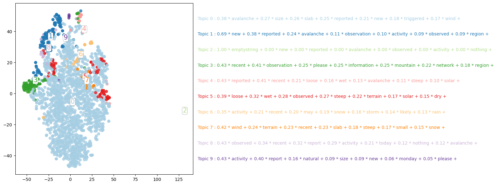
From this plot, we can immediately see two things. First, most documents are closest to topic 0. Second, most topics are not well-separated.

Exercise

See exercise 2 in the exercise list.

Latent Dirichlet Analysis

Latent dirichlet analysis (LDA) produces similar outputs as latent semantic analysis, but LDA often produces nicer results. The statistical theory underlying LSA is built on continuous \(X\) features. LDA uses similar ideas, but takes into account that text is discrete.

# LDA
import gensim
# gensim works with a list of lists of tokens
text_data = [text_prep(txt) for txt in forecasts.avalancheSummary]

# convert to bag of words
dictionary = gensim.corpora.Dictionary(text_data)
bow_data = [dictionary.doc2bow(text) for text in text_data]

ldamodel = gensim.models.ldamodel.LdaModel(bow_data, num_topics = 5, id2word=dictionary, passes=15)
topics = ldamodel.print_topics(num_words=10)
for topic in topics:
    print(topic)

(0, '0.095*"avalanche" + 0.057*"new" + 0.050*"observation" + 0.049*"reported" + 0.036*"mountain" + 0.033*"information" + 0.032*"region" + 0.025*"network" + 0.024*"observed" + 0.023*"activity"')
(1, '0.053*"avalanche" + 0.043*"size" + 0.038*"slab" + 0.030*"triggered" + 0.020*"persistent" + 0.019*"aspect" + 0.017*"layer" + 0.016*"report" + 0.014*"natural" + 0.013*"storm"')
(2, '0.060*"avalanche" + 0.027*"slab" + 0.025*"snow" + 0.025*"storm" + 0.024*"wind" + 0.023*"activity" + 0.022*"new" + 0.020*"may" + 0.017*"likely" + 0.013*"temperature"')
(3, '0.026*"avalanche" + 0.023*"snow" + 0.019*"large" + 0.019*"snowpack" + 0.015*"slab" + 0.013*"consequence" + 0.012*"problem" + 0.011*"valley" + 0.010*"path" + 0.010*"last"')
(4, '0.056*"size" + 0.052*"slab" + 0.051*"avalanche" + 0.029*"loose" + 0.028*"wind" + 0.026*"aspect" + 0.025*"natural" + 0.025*"reported" + 0.020*"triggered" + 0.019*"steep"')

import pyLDAvis
import pyLDAvis.gensim_models
pyLDAvis.enable_notebook()
lda_display = pyLDAvis.gensim_models.prepare(ldamodel, bow_data, dictionary)
lda_display

/home/runner/miniconda3/envs/lecture-datascience/lib/python3.12/site-packages/joblib/externals/loky/backend/fork_exec.py:38: DeprecationWarning: This process (pid=2801) is multi-threaded, use of fork() may lead to deadlocks in the child.
  pid = os.fork()

/home/runner/miniconda3/envs/lecture-datascience/lib/python3.12/site-packages/joblib/externals/loky/backend/fork_exec.py:38: DeprecationWarning: This process (pid=2801) is multi-threaded, use of fork() may lead to deadlocks in the child.
  pid = os.fork()

/home/runner/miniconda3/envs/lecture-datascience/lib/python3.12/site-packages/joblib/externals/loky/backend/fork_exec.py:38: DeprecationWarning: This process (pid=2801) is multi-threaded, use of fork() may lead to deadlocks in the child.
  pid = os.fork()

/home/runner/miniconda3/envs/lecture-datascience/lib/python3.12/site-packages/joblib/externals/loky/backend/fork_exec.py:38: DeprecationWarning: This process (pid=2801) is multi-threaded, use of fork() may lead to deadlocks in the child.
  pid = os.fork()

/home/runner/miniconda3/envs/lecture-datascience/lib/python3.12/site-packages/joblib/externals/loky/backend/fork_exec.py:38: DeprecationWarning: This process (pid=2801) is multi-threaded, use of fork() may lead to deadlocks in the child.
  pid = os.fork()

Exercise

See exercise 3 in the exercise list.

Exercise

See exercise 4 in the exercise list.

Exercises

Exercise 1

Use another classification method to predict incidents. Check whether your method outperforms the Naive Bayes classifier.

(back to text)

Exercise 2

Apply LSA to the weather or snowpack descriptions. Can you notice any patterns?

(back to text)

Exercise 3

Apply LDA to the weather or snowpack descriptions. Can you notice any patterns?

(back to text)

Exercise 4

Use the reduced rank representation of text from LSA or LDA as a feature matrix to predict avalanche incidents. Compare the performance with the bag of words feature matrix.

(back to text)