Time series#
Co-author
Prerequisites
Outcomes
Know how pandas handles dates
Understand how to parse strings into
datetimeobjectsKnow how to write dates as custom formatted strings
Be able to access day, month, year, etc. for a
DateTimeIndexand a column withdtypedatetimeUnderstand both rolling and re-sampling operations and the difference between the two
Data
Bitcoin to USD exchange rates from March 2014 to the present
# Uncomment following line to install on colab
#! pip install
import os
# see section on API keys at end of lecture!
import pandas as pd
import matplotlib.pyplot as plt
import nasdaqdatalink as ndl

ndl.ApiConfig.api_key = os.environ.get("NASDAQ_DATA_LINK_API_KEY", "jEKP58z7JaX6utPkkpEp")

start_date = "2014-05-01"

%matplotlib inline
Intro#
pandas has extensive support for handling dates and times.
We will loosely refer to data with date or time information as time series data.
In this lecture, we will cover the most useful parts of pandas’ time series functionality.
Among these topics are:
Parsing strings as dates
Writing
datetimeobjects as strings (inverse operation of previous point)Extracting data from a DataFrame or Series with date information in the index
Shifting data through time (taking leads or lags)
Re-sampling data to a different frequency and rolling operations
However, even more than with previous topics, we will skip a lot of the functionality pandas offers, and we urge you to refer to the official documentation for more information.
Parsing Strings as Dates#
When working with time series data, we almost always receive the data with dates encoded as strings.
Hopefully, the date strings follow a structured format or pattern.
One common pattern is YYYY-MM-DD: 4 numbers for the year, 2 for the
month, and 2 for the day with each section separated by a -.
For example, we write Christmas day 2017 in this format as
christmas_str = "2017-12-25"
To convert a string into a time-aware object, we use the
pd.to_datetime function.
christmas = pd.to_datetime(christmas_str)
print("The type of christmas is", type(christmas))
christmas
The type of christmas is <class 'pandas._libs.tslibs.timestamps.Timestamp'>
Timestamp('2017-12-25 00:00:00')
The pd.to_datetime function is pretty smart at guessing the format
of the date…
for date in ["December 25, 2017", "Dec. 25, 2017",
             "Monday, Dec. 25, 2017", "25 Dec. 2017", "25th Dec. 2017"]:
    print("pandas interprets {} as {}".format(date, pd.to_datetime(date)))
pandas interprets December 25, 2017 as 2017-12-25 00:00:00
pandas interprets Dec. 25, 2017 as 2017-12-25 00:00:00
pandas interprets Monday, Dec. 25, 2017 as 2017-12-25 00:00:00
pandas interprets 25 Dec. 2017 as 2017-12-25 00:00:00
pandas interprets 25th Dec. 2017 as 2017-12-25 00:00:00
However, sometimes we will need to give pandas a hint.
For example, that same time (midnight on Christmas) would be reported on an Amazon transaction report as
christmas_amzn = "2017-12-25T00:00:00+ 00 :00"
If we try to pass this to pd.to_datetime, it will fail.
pd.to_datetime(christmas_amzn)
---------------------------------------------------------------------------
DateParseError                            Traceback (most recent call last)
Cell In[6], line 1
----> 1 pd.to_datetime(christmas_amzn)

File ~/miniconda3/envs/lecture-datascience/lib/python3.12/site-packages/pandas/core/tools/datetimes.py:1101, in to_datetime(arg, errors, dayfirst, yearfirst, utc, format, exact, unit, infer_datetime_format, origin, cache)
   1099         result = convert_listlike(argc, format)
   1100 else:
-> 1101     result = convert_listlike(np.array([arg]), format)[0]
   1102     if isinstance(arg, bool) and isinstance(result, np.bool_):
   1103         result = bool(result)  # TODO: avoid this kludge.

File ~/miniconda3/envs/lecture-datascience/lib/python3.12/site-packages/pandas/core/tools/datetimes.py:435, in _convert_listlike_datetimes(arg, format, name, utc, unit, errors, dayfirst, yearfirst, exact)
    432 if format is not None and format != "mixed":
    433     return _array_strptime_with_fallback(arg, name, utc, format, exact, errors)
--> 435 result, tz_parsed = objects_to_datetime64(
    436     arg,
    437     dayfirst=dayfirst,
    438     yearfirst=yearfirst,
    439     utc=utc,
    440     errors=errors,
    441     allow_object=True,
    442 )
    444 if tz_parsed is not None:
    445     # We can take a shortcut since the datetime64 numpy array
    446     # is in UTC
    447     out_unit = np.datetime_data(result.dtype)[0]

File ~/miniconda3/envs/lecture-datascience/lib/python3.12/site-packages/pandas/core/arrays/datetimes.py:2398, in objects_to_datetime64(data, dayfirst, yearfirst, utc, errors, allow_object, out_unit)
   2395 # if str-dtype, convert
   2396 data = np.asarray(data, dtype=np.object_)
-> 2398 result, tz_parsed = tslib.array_to_datetime(
   2399     data,
   2400     errors=errors,
   2401     utc=utc,
   2402     dayfirst=dayfirst,
   2403     yearfirst=yearfirst,
   2404     creso=abbrev_to_npy_unit(out_unit),
   2405 )
   2407 if tz_parsed is not None:
   2408     # We can take a shortcut since the datetime64 numpy array
   2409     #  is in UTC
   2410     return result, tz_parsed

File tslib.pyx:414, in pandas._libs.tslib.array_to_datetime()

File tslib.pyx:596, in pandas._libs.tslib.array_to_datetime()

File tslib.pyx:553, in pandas._libs.tslib.array_to_datetime()

File conversion.pyx:641, in pandas._libs.tslibs.conversion.convert_str_to_tsobject()

File parsing.pyx:336, in pandas._libs.tslibs.parsing.parse_datetime_string()

File parsing.pyx:666, in pandas._libs.tslibs.parsing.dateutil_parse()

DateParseError: Unknown datetime string format, unable to parse: 2017-12-25T00:00:00+ 00 :00, at position 0
To parse a date with this format, we need to specify the format
argument for pd.to_datetime.
amzn_strftime = "%Y-%m-%dT%H:%M:%S+ 00 :00"
pd.to_datetime(christmas_amzn, format=amzn_strftime)
Timestamp('2017-12-25 00:00:00')
Can you guess what amzn_strftime represents?
Let’s take a closer look at amzn_strftime and christmas_amzn.
print(amzn_strftime)
print(christmas_amzn)
%Y-%m-%dT%H:%M:%S+ 00 :00
2017-12-25T00:00:00+ 00 :00
Notice that both of the strings have a similar form, but that instead of actual numerical values, amzn_strftime has placeholders.
Specifically, anywhere the % shows up is a signal to the pd.to_datetime
function that it is where relevant information is stored.
For example, the %Y is a stand-in for a four digit year, %m is
for 2 a digit month, and so on…
The official Python
documentation contains a complete list of possible %something patterns that are accepted
in the format argument.
Exercise
See exercise 1 in the exercise list.
Multiple Dates#
If we have dates in a Series (e.g. column of DataFrame) or a list, we
can pass the entire collection to pd.to_datetime and get a
collection of dates back.
We’ll just show an example of that here as the mechanics are the same as a single date.
pd.to_datetime(["2017-12-25", "2017-12-31"])
DatetimeIndex(['2017-12-25', '2017-12-31'], dtype='datetime64[ns]', freq=None)
Date Formatting#
We can use the %pattern format to have pandas write datetime
objects as specially formatted strings using the strftime (string
format time) method.
For example,
christmas.strftime("We love %A %B %d (also written %c)")
'We love Monday December 25 (also written Mon Dec 25 00:00:00 2017)'
Exercise
See exercise 2 in the exercise list.
Extracting Data#
When the index of a DataFrame has date information and pandas
recognizes the values as datetime values, we can leverage some
convenient indexing features for extracting data.
The flexibility of these features is best understood through example, so let’s load up some data and take a look.
btc_usd_long = ndl.get_table("QDL/BCHAIN", date = { 'gte': '2009-12-25', 'lte': '2019-01-01' }, code = ["MKPRU", "MKTCP", "ETRVU"])
btc_usd_long.info()
btc_usd_long.head()
<class 'pandas.core.frame.DataFrame'>
RangeIndex: 9885 entries, 0 to 9884
Data columns (total 3 columns):
 #   Column  Non-Null Count  Dtype
---  ------  --------------  -----
 0   code    9885 non-null   object
 1   date    9885 non-null   datetime64[ns]
 2   value   9885 non-null   float64
dtypes: datetime64[ns](1), float64(1), object(1)
memory usage: 231.8+ KB
| code | date | value | |
|---|---|---|---|
| None | |||
| 0 | MKTCP | 2019-01-01 | 6.550566e+10 |
| 1 | MKTCP | 2018-12-31 | 6.638886e+10 |
| 2 | MKTCP | 2018-12-30 | 6.689905e+10 |
| 3 | MKTCP | 2018-12-29 | 6.827565e+10 |
| 4 | MKTCP | 2018-12-28 | 6.709189e+10 |
Here, we have the Bitcoin (BTC) to US dollar (USD) exchange rate from 2009 until today, as well as other variables relevant to the Bitcoin ecosystem, in long (“melted”) form.
print(btc_usd_long.code.unique())
btc_usd_long.dtypes
['MKTCP' 'MKPRU' 'ETRVU']
code             object
date     datetime64[ns]
value           float64
dtype: object
Notice that the type of date is datetime. We would like this to be the index, and we want to drop the long form. We also selected only a couple of columns of interest, but the dataset has a lot more options. (The column descriptions can be found here). We chose Market Price (in USD) (MKPRU), Total Market Cap (MKTCP), and Estimated Transaction Volume in USD (ETRVU).
btc_usd = btc_usd_long.pivot_table(index='date', columns='code', values='value')
btc_usd.head()
| code | ETRVU | MKPRU | MKTCP |
|---|---|---|---|
| date | |||
| 2009-12-25 | 0.0 | 0.0 | 0.0 |
| 2009-12-26 | 0.0 | 0.0 | 0.0 |
| 2009-12-27 | 0.0 | 0.0 | 0.0 |
| 2009-12-28 | 0.0 | 0.0 | 0.0 |
| 2009-12-29 | 0.0 | 0.0 | 0.0 |
Now that we have a datetime index, it enables things like…
Extracting all data for the year 2015 by passing "2015" to .loc.
btc_usd.loc["2015"]
| code | ETRVU | MKPRU | MKTCP |
|---|---|---|---|
| date | |||
| 2015-01-01 | 2.831524e+07 | 316.15 | 4.388454e+09 |
| 2015-01-02 | 5.458287e+07 | 314.81 | 4.136728e+09 |
| 2015-01-03 | 9.035606e+07 | 270.93 | 3.708212e+09 |
| 2015-01-04 | 6.263383e+07 | 276.80 | 3.901250e+09 |
| 2015-01-05 | 5.647246e+07 | 263.17 | 3.790804e+09 |
| ... | ... | ... | ... |
| 2015-12-27 | 7.700877e+07 | 418.46 | 6.420190e+09 |
| 2015-12-28 | 1.057652e+08 | 422.42 | 6.366855e+09 |
| 2015-12-29 | 1.158679e+08 | 431.13 | 6.475864e+09 |
| 2015-12-30 | 9.992696e+07 | 428.00 | 6.386794e+09 |
| 2015-12-31 | 7.566080e+07 | 428.23 | 6.452379e+09 |
365 rows × 3 columns
We can also narrow down to specific months.
# By month's name
btc_usd.loc["August 2017"]
| code | ETRVU | MKPRU | MKTCP |
|---|---|---|---|
| date | |||
| 2017-08-01 | 1.369196e+09 | 2862.9000 | 4.550093e+10 |
| 2017-08-02 | 1.424506e+09 | 2693.6340 | 4.440385e+10 |
| 2017-08-03 | 9.709563e+08 | 2794.1177 | 4.606512e+10 |
| 2017-08-04 | 1.196485e+09 | 2790.0000 | 4.631086e+10 |
| 2017-08-05 | 9.791541e+08 | 3218.1150 | 5.306965e+10 |
| 2017-08-06 | 1.044204e+09 | 3252.5625 | 5.364342e+10 |
| 2017-08-07 | 1.385571e+09 | 3210.2000 | 5.319216e+10 |
| 2017-08-08 | 1.230026e+09 | 3457.3743 | 5.703501e+10 |
| 2017-08-09 | 8.071196e+08 | 3357.3263 | 5.526816e+10 |
| 2017-08-10 | 9.631284e+08 | 3340.2800 | 5.650275e+10 |
| 2017-08-11 | 9.856015e+08 | 3632.5067 | 5.994299e+10 |
| 2017-08-12 | 8.706294e+08 | 3852.8029 | 6.358478e+10 |
| 2017-08-13 | 9.264450e+08 | 3868.5200 | 6.693611e+10 |
| 2017-08-14 | 8.666749e+08 | 4282.9920 | 7.069930e+10 |
| 2017-08-15 | 1.206088e+09 | 4217.0283 | 6.961845e+10 |
| 2017-08-16 | 9.825228e+08 | 4179.9700 | 6.764231e+10 |
| 2017-08-17 | 1.362841e+09 | 4328.7257 | 7.147917e+10 |
| 2017-08-18 | 1.137242e+09 | 4130.4401 | 6.821262e+10 |
| 2017-08-19 | 1.323689e+09 | 4104.7100 | 6.812422e+10 |
| 2017-08-20 | 7.589911e+08 | 4157.9580 | 6.868167e+10 |
| 2017-08-21 | 8.194572e+08 | 4043.7220 | 6.680052e+10 |
| 2017-08-22 | 8.814776e+08 | 3986.2800 | 6.755553e+10 |
| 2017-08-23 | 1.053264e+09 | 4174.9500 | 6.898129e+10 |
| 2017-08-24 | 7.560436e+08 | 4340.3167 | 7.171907e+10 |
| 2017-08-25 | 7.651743e+08 | 4331.7700 | 7.210029e+10 |
| 2017-08-26 | 6.879348e+08 | 4360.5133 | 7.067509e+10 |
| 2017-08-27 | 7.814597e+08 | 4354.3083 | 7.196991e+10 |
| 2017-08-28 | 9.251545e+08 | 4339.0500 | 7.259458e+10 |
| 2017-08-29 | 1.113344e+09 | 4607.9854 | 7.593083e+10 |
| 2017-08-30 | 1.010876e+09 | 4594.9879 | 7.597359e+10 |
| 2017-08-31 | 1.192190e+09 | 4582.5200 | 7.851738e+10 |
# By month's number
btc_usd.loc["08/2017"]
| code | ETRVU | MKPRU | MKTCP |
|---|---|---|---|
| date | |||
| 2017-08-01 | 1.369196e+09 | 2862.9000 | 4.550093e+10 |
| 2017-08-02 | 1.424506e+09 | 2693.6340 | 4.440385e+10 |
| 2017-08-03 | 9.709563e+08 | 2794.1177 | 4.606512e+10 |
| 2017-08-04 | 1.196485e+09 | 2790.0000 | 4.631086e+10 |
| 2017-08-05 | 9.791541e+08 | 3218.1150 | 5.306965e+10 |
| 2017-08-06 | 1.044204e+09 | 3252.5625 | 5.364342e+10 |
| 2017-08-07 | 1.385571e+09 | 3210.2000 | 5.319216e+10 |
| 2017-08-08 | 1.230026e+09 | 3457.3743 | 5.703501e+10 |
| 2017-08-09 | 8.071196e+08 | 3357.3263 | 5.526816e+10 |
| 2017-08-10 | 9.631284e+08 | 3340.2800 | 5.650275e+10 |
| 2017-08-11 | 9.856015e+08 | 3632.5067 | 5.994299e+10 |
| 2017-08-12 | 8.706294e+08 | 3852.8029 | 6.358478e+10 |
| 2017-08-13 | 9.264450e+08 | 3868.5200 | 6.693611e+10 |
| 2017-08-14 | 8.666749e+08 | 4282.9920 | 7.069930e+10 |
| 2017-08-15 | 1.206088e+09 | 4217.0283 | 6.961845e+10 |
| 2017-08-16 | 9.825228e+08 | 4179.9700 | 6.764231e+10 |
| 2017-08-17 | 1.362841e+09 | 4328.7257 | 7.147917e+10 |
| 2017-08-18 | 1.137242e+09 | 4130.4401 | 6.821262e+10 |
| 2017-08-19 | 1.323689e+09 | 4104.7100 | 6.812422e+10 |
| 2017-08-20 | 7.589911e+08 | 4157.9580 | 6.868167e+10 |
| 2017-08-21 | 8.194572e+08 | 4043.7220 | 6.680052e+10 |
| 2017-08-22 | 8.814776e+08 | 3986.2800 | 6.755553e+10 |
| 2017-08-23 | 1.053264e+09 | 4174.9500 | 6.898129e+10 |
| 2017-08-24 | 7.560436e+08 | 4340.3167 | 7.171907e+10 |
| 2017-08-25 | 7.651743e+08 | 4331.7700 | 7.210029e+10 |
| 2017-08-26 | 6.879348e+08 | 4360.5133 | 7.067509e+10 |
| 2017-08-27 | 7.814597e+08 | 4354.3083 | 7.196991e+10 |
| 2017-08-28 | 9.251545e+08 | 4339.0500 | 7.259458e+10 |
| 2017-08-29 | 1.113344e+09 | 4607.9854 | 7.593083e+10 |
| 2017-08-30 | 1.010876e+09 | 4594.9879 | 7.597359e+10 |
| 2017-08-31 | 1.192190e+09 | 4582.5200 | 7.851738e+10 |
Or even a day…
# By date name
btc_usd.loc["August 1, 2017"]
code
ETRVU    1.369196e+09
MKPRU    2.862900e+03
MKTCP    4.550093e+10
Name: 2017-08-01 00:00:00, dtype: float64
# By date number
btc_usd.loc["08-01-2017"]
code
ETRVU    1.369196e+09
MKPRU    2.862900e+03
MKTCP    4.550093e+10
Name: 2017-08-01 00:00:00, dtype: float64
What can we pass as the .loc argument when we have a
DateTimeIndex?
Anything that can be converted to a datetime using
pd.to_datetime, without having to specify the format argument.
When that condition holds, pandas will return all rows whose date in the index “belong” to that date or period.
We can also use the range shorthand notation to give a start and end date for selection.
btc_usd.loc["April 1, 2015":"April 10, 2015"]
| code | ETRVU | MKPRU | MKTCP |
|---|---|---|---|
| date | |||
| 2015-04-01 | 5.354486e+07 | 252.44 | 3.536773e+09 |
| 2015-04-02 | 4.016409e+07 | 246.49 | 3.565053e+09 |
| 2015-04-03 | 4.331351e+07 | 253.77 | 3.549561e+09 |
| 2015-04-04 | 2.205524e+07 | 257.03 | 3.604010e+09 |
| 2015-04-05 | 2.832354e+07 | 253.67 | 3.572161e+09 |
| 2015-04-06 | 3.991755e+07 | 255.48 | 3.584116e+09 |
| 2015-04-07 | 5.134161e+07 | 245.89 | 3.579212e+09 |
| 2015-04-08 | 5.092222e+07 | 253.90 | 3.438417e+09 |
| 2015-04-09 | 5.215728e+07 | 235.71 | 3.309144e+09 |
| 2015-04-10 | 4.316281e+07 | 236.70 | 3.411246e+09 |
Exercise
See exercise 3 in the exercise list.
Accessing Date Properties#
Sometimes, we would like to directly access a part of the date/time.
If our date/time information is in the index, we can to df.index.XX
where XX is replaced by year, month, or whatever we would
like to access.
btc_usd.index.year
Index([2009, 2009, 2009, 2009, 2009, 2009, 2009, 2010, 2010, 2010,
       ...
       2018, 2018, 2018, 2018, 2018, 2018, 2018, 2018, 2018, 2019],
      dtype='int32', name='date', length=3295)
btc_usd.index.day
Index([25, 26, 27, 28, 29, 30, 31,  1,  2,  3,
       ...
       23, 24, 25, 26, 27, 28, 29, 30, 31,  1],
      dtype='int32', name='date', length=3295)
We can also do the same if the date/time information is stored in a column, but we have to use a slightly different syntax.
df["column_name"].dt.XX
btc_date_column = btc_usd.reset_index()
btc_date_column.head()
| code | date | ETRVU | MKPRU | MKTCP |
|---|---|---|---|---|
| 0 | 2009-12-25 | 0.0 | 0.0 | 0.0 |
| 1 | 2009-12-26 | 0.0 | 0.0 | 0.0 |
| 2 | 2009-12-27 | 0.0 | 0.0 | 0.0 |
| 3 | 2009-12-28 | 0.0 | 0.0 | 0.0 |
| 4 | 2009-12-29 | 0.0 | 0.0 | 0.0 |
btc_date_column["date"].dt.year.head()
0    2009
1    2009
2    2009
3    2009
4    2009
Name: date, dtype: int32
btc_date_column["date"].dt.month.head()
0    12
1    12
2    12
3    12
4    12
Name: date, dtype: int32
Leads and Lags: df.shift#
When doing time series analysis, we often want to compare data at one date against data at another date.
pandas can help us with this if we leverage the shift method.
Without any additional arguments, shift() will move all data
forward one period, filling the first row with missing data.
# so we can see the result of shift clearly
btc_usd.head()
| code | ETRVU | MKPRU | MKTCP |
|---|---|---|---|
| date | |||
| 2009-12-25 | 0.0 | 0.0 | 0.0 |
| 2009-12-26 | 0.0 | 0.0 | 0.0 |
| 2009-12-27 | 0.0 | 0.0 | 0.0 |
| 2009-12-28 | 0.0 | 0.0 | 0.0 |
| 2009-12-29 | 0.0 | 0.0 | 0.0 |
btc_usd.shift().head()
| code | ETRVU | MKPRU | MKTCP |
|---|---|---|---|
| date | |||
| 2009-12-25 | NaN | NaN | NaN |
| 2009-12-26 | 0.0 | 0.0 | 0.0 |
| 2009-12-27 | 0.0 | 0.0 | 0.0 |
| 2009-12-28 | 0.0 | 0.0 | 0.0 |
| 2009-12-29 | 0.0 | 0.0 | 0.0 |
We can use this to compute the percent change from one day to the next. (Quiz: Why does that work? Remember how pandas uses the index to align data.)
((btc_usd - btc_usd.shift()) / btc_usd.shift()).head()
| code | ETRVU | MKPRU | MKTCP |
|---|---|---|---|
| date | |||
| 2009-12-25 | NaN | NaN | NaN |
| 2009-12-26 | NaN | NaN | NaN |
| 2009-12-27 | NaN | NaN | NaN |
| 2009-12-28 | NaN | NaN | NaN |
| 2009-12-29 | NaN | NaN | NaN |
Setting the first argument to n tells pandas to shift the data down
n rows (apply an n period lag).
btc_usd.shift(3).head()
| code | ETRVU | MKPRU | MKTCP |
|---|---|---|---|
| date | |||
| 2009-12-25 | NaN | NaN | NaN |
| 2009-12-26 | NaN | NaN | NaN |
| 2009-12-27 | NaN | NaN | NaN |
| 2009-12-28 | 0.0 | 0.0 | 0.0 |
| 2009-12-29 | 0.0 | 0.0 | 0.0 |
A negative value will shift the data up or apply a lead.
btc_usd.shift(-2).head()
| code | ETRVU | MKPRU | MKTCP |
|---|---|---|---|
| date | |||
| 2009-12-25 | 0.0 | 0.0 | 0.0 |
| 2009-12-26 | 0.0 | 0.0 | 0.0 |
| 2009-12-27 | 0.0 | 0.0 | 0.0 |
| 2009-12-28 | 0.0 | 0.0 | 0.0 |
| 2009-12-29 | 0.0 | 0.0 | 0.0 |
btc_usd.shift(-2).tail()
| code | ETRVU | MKPRU | MKTCP |
|---|---|---|---|
| date | |||
| 2018-12-28 | 2.700024e+08 | 3770.3600 | 6.689905e+10 |
| 2018-12-29 | 4.760031e+08 | 3791.5458 | 6.638886e+10 |
| 2018-12-30 | 2.236265e+08 | 3752.2717 | 6.550566e+10 |
| 2018-12-31 | NaN | NaN | NaN |
| 2019-01-01 | NaN | NaN | NaN |
Exercise
See exercise 4 in the exercise list.
Rolling Computations: .rolling#
pandas has facilities that enable easy computation of rolling statistics.
These are best understood by example, so we will dive right in.
# first take only the first 6 rows so we can easily see what is going on
btc_small = btc_usd.head(6)
btc_small
| code | ETRVU | MKPRU | MKTCP |
|---|---|---|---|
| date | |||
| 2009-12-25 | 0.0 | 0.0 | 0.0 |
| 2009-12-26 | 0.0 | 0.0 | 0.0 |
| 2009-12-27 | 0.0 | 0.0 | 0.0 |
| 2009-12-28 | 0.0 | 0.0 | 0.0 |
| 2009-12-29 | 0.0 | 0.0 | 0.0 |
| 2009-12-30 | 0.0 | 0.0 | 0.0 |
Below, we compute the 2 day moving average (for all columns).
btc_small.rolling("2d").mean()
| code | ETRVU | MKPRU | MKTCP |
|---|---|---|---|
| date | |||
| 2009-12-25 | 0.0 | 0.0 | 0.0 |
| 2009-12-26 | 0.0 | 0.0 | 0.0 |
| 2009-12-27 | 0.0 | 0.0 | 0.0 |
| 2009-12-28 | 0.0 | 0.0 | 0.0 |
| 2009-12-29 | 0.0 | 0.0 | 0.0 |
| 2009-12-30 | 0.0 | 0.0 | 0.0 |
To do this operation, pandas starts at each row (date) then looks
backwards the specified number of periods (here 2 days) and then
applies some aggregation function (mean) on all the data in that
window.
If pandas cannot look back the full length of the window (e.g. when working on the first row), it fills as much of the window as possible and then does the operation. Notice that the value at 2014-05-01 is the same in both DataFrames.
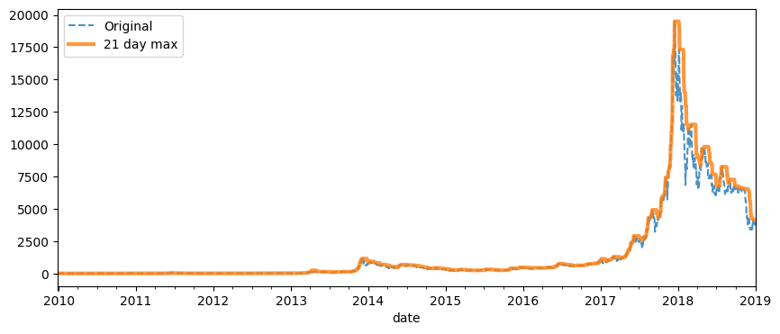
Below, we see a visual depiction of the rolling maximum on a 21 day window for the whole dataset.
fig, ax = plt.subplots(figsize=(10, 4))
btc_usd["MKPRU"].plot(ax=ax, linestyle="--", alpha=0.8)
btc_usd.rolling("21d").max()["MKPRU"].plot(ax=ax, alpha=0.8, linewidth=3)
ax.legend(["Original", "21 day max"])
<matplotlib.legend.Legend at 0x7fe232d81ac0>
We can also ask pandas to apply custom functions, similar to what we
saw when studying GroupBy.
def is_volatile(x):
    "Returns a 1 if the variance is greater than 1, otherwise returns 0"
    if x.var() > 1.0:
        return 1.0
    else:
        return 0.0
btc_small.rolling("2d").apply(is_volatile)
| code | ETRVU | MKPRU | MKTCP |
|---|---|---|---|
| date | |||
| 2009-12-25 | 0.0 | 0.0 | 0.0 |
| 2009-12-26 | 0.0 | 0.0 | 0.0 |
| 2009-12-27 | 0.0 | 0.0 | 0.0 |
| 2009-12-28 | 0.0 | 0.0 | 0.0 |
| 2009-12-29 | 0.0 | 0.0 | 0.0 |
| 2009-12-30 | 0.0 | 0.0 | 0.0 |
Exercise
See exercise 5 in the exercise list.
To make the optimal decision, we need to know the maximum difference between the close price at the end of the window and the open price at the start of the window.
Exercise
See exercise 6 in the exercise list.
Changing Frequencies: .resample#
In addition to computing rolling statistics, we can also change the frequency of the data.
For example, instead of a monthly moving average, suppose that we wanted to compute the average within each calendar month.
We will use the resample method to do this.
Below are some examples.
# business quarter
btc_usd.resample("BQE").mean()
| code | ETRVU | MKPRU | MKTCP |
|---|---|---|---|
| date | |||
| 2009-12-31 | 0.000000e+00 | 0.000000 | 0.000000e+00 |
| 2010-03-31 | 0.000000e+00 | 0.000000 | 0.000000e+00 |
| 2010-06-30 | 0.000000e+00 | 0.000000 | 0.000000e+00 |
| 2010-09-30 | 8.522276e+02 | 0.033260 | 1.317223e+05 |
| 2010-12-31 | 1.179063e+04 | 0.217938 | 1.015812e+06 |
| 2011-03-31 | 4.516475e+04 | 0.737402 | 4.043357e+06 |
| 2011-06-30 | 1.729951e+06 | 9.176310 | 5.956523e+07 |
| 2011-09-30 | 9.176091e+05 | 10.742849 | 7.522893e+07 |
| 2011-12-30 | 1.991838e+06 | 3.419525 | 2.639635e+07 |
| 2012-03-30 | 7.588531e+05 | 5.592202 | 4.670274e+07 |
| 2012-06-29 | 1.101213e+06 | 5.407497 | 4.886157e+07 |
| 2012-09-28 | 2.821250e+06 | 10.356359 | 1.007798e+08 |
| 2012-12-31 | 2.701674e+06 | 12.368074 | 1.286258e+08 |
| 2013-03-29 | 8.611094e+06 | 32.621256 | 3.515062e+08 |
| 2013-06-28 | 2.782766e+07 | 119.419551 | 1.337195e+09 |
| 2013-09-30 | 1.979282e+07 | 107.674014 | 1.242022e+09 |
| 2013-12-31 | 1.081436e+08 | 494.289457 | 6.009161e+09 |
| 2014-03-31 | 9.001297e+07 | 693.245444 | 8.591035e+09 |
| 2014-06-30 | 5.479866e+07 | 520.799451 | 6.665094e+09 |
| 2014-09-30 | 5.296835e+07 | 534.162283 | 7.020311e+09 |
| 2014-12-31 | 6.272862e+07 | 357.784674 | 4.835176e+09 |
| 2015-03-31 | 5.113746e+07 | 250.173111 | 3.481522e+09 |
| 2015-06-30 | 4.752748e+07 | 236.218681 | 3.355567e+09 |
| 2015-09-30 | 6.545561e+07 | 255.963913 | 3.712326e+09 |
| 2015-12-31 | 1.385931e+08 | 345.638152 | 5.142968e+09 |
| 2016-03-31 | 1.283647e+08 | 409.983516 | 6.226075e+09 |
| 2016-06-30 | 1.665296e+08 | 510.586051 | 7.972975e+09 |
| 2016-09-30 | 1.499507e+08 | 615.694674 | 9.752593e+09 |
| 2016-12-30 | 1.928515e+08 | 724.429451 | 1.163821e+10 |
| 2017-03-31 | 2.747348e+08 | 1033.310616 | 1.667005e+10 |
| 2017-06-30 | 5.764680e+08 | 1900.426105 | 3.122785e+10 |
| 2017-09-29 | 8.735033e+08 | 3461.377390 | 5.764089e+10 |
| 2017-12-29 | 2.332756e+09 | 9258.879054 | 1.552192e+11 |
| 2018-03-30 | 1.906414e+09 | 10664.432624 | 1.792487e+11 |
| 2018-06-29 | 9.201284e+08 | 7787.273765 | 1.320632e+11 |
| 2018-09-28 | 7.135467e+08 | 6797.888576 | 1.170264e+11 |
| 2018-12-31 | 7.343926e+08 | 5248.198650 | 9.075620e+10 |
| 2019-03-29 | 2.236265e+08 | 3752.271700 | 6.550566e+10 |
Note that unlike with rolling, a single number is returned for
each column for each quarter.
The resample method will alter the frequency of the data and the
number of rows in the result will be different from the number of rows
in the input.
On the other hand, with rolling, the size and frequency of the result
are the same as the input.
We can sample at other frequencies and aggregate with multiple aggregations function at once.
# multiple functions at 2 start-of-quarter frequency
btc_usd.resample("2BQS").agg(["min", "max"])
| code | ETRVU | MKPRU | MKTCP | |||
|---|---|---|---|---|---|---|
| min | max | min | max | min | max | |
| date | ||||||
| 2009-10-01 | 0.000000e+00 | 0.000000e+00 | 0.0000 | 0.0000 | 0.000000e+00 | 0.000000e+00 |
| 2010-04-01 | 0.000000e+00 | 4.780000e+03 | 0.0000 | 0.1750 | 0.000000e+00 | 6.992825e+05 |
| 2010-10-01 | 1.649000e+03 | 2.441970e+05 | 0.0600 | 1.1000 | 2.493210e+05 | 5.901940e+06 |
| 2011-04-01 | 2.740300e+04 | 1.815384e+07 | 0.7100 | 35.0000 | 4.150234e+06 | 2.272585e+08 |
| 2011-10-03 | 1.975250e+05 | 1.637516e+07 | 2.2900 | 7.2200 | 1.766128e+07 | 5.811768e+07 |
| 2012-04-02 | 4.122260e+05 | 1.322970e+07 | 4.8000 | 15.4000 | 4.195824e+07 | 1.496572e+08 |
| 2012-10-01 | 7.742860e+05 | 2.769433e+07 | 10.6010 | 93.5670 | 1.093527e+08 | 1.125488e+09 |
| 2013-04-01 | 9.821585e+06 | 1.385370e+08 | 67.8584 | 237.9900 | 7.519925e+08 | 2.620841e+09 |
| 2013-10-01 | 1.150644e+07 | 3.843574e+08 | 103.8500 | 1151.0000 | 1.230957e+09 | 1.350490e+10 |
| 2014-04-01 | 1.976148e+07 | 1.765106e+08 | 380.0000 | 673.9000 | 4.661392e+09 | 8.668279e+09 |
| 2014-10-01 | 2.502690e+07 | 1.781682e+08 | 176.5000 | 430.0700 | 2.707305e+09 | 5.802913e+09 |
| 2015-04-01 | 2.205524e+07 | 1.056422e+08 | 216.0000 | 310.5500 | 3.077795e+09 | 4.464575e+09 |
| 2015-10-01 | 4.002130e+07 | 3.353970e+08 | 237.7800 | 463.9800 | 3.486830e+09 | 6.952138e+09 |
| 2016-04-01 | 7.246670e+07 | 4.338279e+08 | 416.2500 | 754.3600 | 6.402758e+09 | 1.212991e+10 |
| 2016-10-03 | 1.006182e+08 | 5.526767e+08 | 607.1800 | 1287.0000 | 9.676305e+09 | 2.089075e+10 |
| 2017-04-03 | 1.955462e+08 | 1.772644e+09 | 1079.9900 | 4911.7400 | 1.846992e+10 | 7.969529e+10 |
| 2017-10-02 | 5.506455e+08 | 5.729890e+09 | 4225.1750 | 19498.6833 | 7.021588e+10 | 3.346692e+11 |
| 2018-04-02 | 2.724822e+08 | 1.986371e+09 | 5908.7025 | 9803.3067 | 1.005508e+11 | 1.668274e+11 |
| 2018-10-01 | 2.236265e+08 | 2.721201e+09 | 3242.4200 | 6626.8500 | 5.620096e+10 | 1.146456e+11 |
As with groupby and rolling, you can also provide custom
functions to .resample(...).agg and .resample(...).apply
Exercise
See exercise 7 in the exercise list.
To make the optimal decision we need to, for each month, compute the maximum value of the close price on any day minus the open price on the first day of the month.
Exercise
See exercise 8 in the exercise list.
Optional: API keys#
Recall above that we had the line of code:
ndl.ApiConfig.api_key = os.environ.get("NASDAQ_DATA_LINK_API_KEY", "jEKP58z7JaX6utPkkpEp")
This line told the nasdaqdatalink library that when obtaining making requests for data, it should use the API key jEKP58z7JaX6utPkkpEp.
An API key is a sort of password that web services (like the Nasdaq Data Link API) require you to provide when you make requests.
Using this password, we were able to make a request to Nasdaq data link to obtain data directly from them.
The API key used here is one that we requested on behalf of this course. If you create your own API key, you should store it in the NASDAQ_DATA_LINK_API_KEY environment variable, locally on your computer. Using an environment variable like this is a common way to store sensitive information like API keys, since you can set the environment variable in a secure way that is not stored in your code. How to set environment variables varies by operating system, but you can find instructions for doing so on the web.
If you plan to use Nasdaq data more extensively, you should obtain your own personal API key from their website and re-run the os.environ... line of code with your new API key on the right-hand side.
Exercises#
Exercise 1#
By referring to table found at the link above, figure out the correct argument to
pass as format in order to parse the dates in the next three cells below.
Test your work by passing your format string to pd.to_datetime.
christmas_str2 = "2017:12:25"
dbacks_win = "M:11 D:4 Y:2001 9:15 PM"
america_bday = "America was born on July 4, 1776"
Exercise 2#
Use pd.to_datetime to express the birthday of one of your friends
or family members as a datetime object.
Then use the strftime method to write a message of the format:
NAME's birthday is June 10, 1989 (a Saturday)
(where the name and date are replaced by the appropriate values)
Exercise 3#
For each item in the list, extract the specified data from btc_usd:
July 2017 through August 2017 (inclusive)
April 25, 2015 to June 10, 2016
October 31, 2017
Exercise 4#
Using the shift function, determine the week with the largest percent change
in the volume of trades (the "Volume (BTC)" column).
Repeat the analysis at the bi-weekly and monthly frequencies.
Hint
We have data at a daily frequency and one week is 7 days.
Hint
Approximate a month by 30 days.
# your code here
Exercise 5#
Imagine that you have access to the DeLorean time machine from “Back to the Future”.
You are allowed to use the DeLorean only once, subject to the following conditions:
You may travel back to any day in the past.
On that day, you may purchase one bitcoin at market open.
You can then take the time machine 30 days into the future and sell your bitcoin at market close.
Then you return to the present, pocketing the profits.
How would you pick the day?
Think carefully about what you would need to compute to make the optimal choice. Try writing it out in the markdown cell below so you have a clear description of the want operator that we will apply after the exercise.
(Note: Don’t look too far below, because in the next non-empty cell we have written out our answer.)
To make this decision, we want to know …
Your answer here
Exercise 6#
Do the following:
Write a pandas function that implements your strategy.
Pass it to the
aggmethod ofrolling_btc.Extract the
"Open"column from the result.Find the date associated with the maximum value in that column.
How much money did you make? Compare with your neighbor.
def daily_value(df):
    # DELETE `pass` below and replace it with your code
    pass

rolling_btc = btc_usd.rolling("30d")

# do steps 2-4 here
Exercise 7#
Now suppose you still have access to the DeLorean, but the conditions are slightly different.
You may now:
Travel back to the first day of any month in the past.
On that day, you may purchase one bitcoin at market open.
You can then travel to any day in that month and sell the bitcoin at market close.
Then return to the present, pocketing the profits.
To which month would you travel? On which day of that month would you return to sell the bitcoin?
Discuss with your neighbor what you would need to compute to make the optimal choice. Try writing it out in the markdown cell below so you have a clear description of the want operator that we will apply after the exercise.
(Note: Don’t look too many cells below, because we have written out our answer.)
To make the optimal decision we need …
Your answer here
Exercise 8#
Do the following:
Write a pandas function that implements your strategy.
Pass it to the
aggmethod ofresampled_btc.Extract the
"Open"column from the result.Find the date associated with the maximum value in that column.
How much money did you make? Compare with your neighbor.
Was this strategy more profitable than the previous one? By how much?
def monthly_value(df):
    # DELETE `pass` below and replace it with your code
    pass

resampled_btc = btc_usd.resample("MS")

# Do steps 2-4 here