Heterogeneous Effects#
Author
Prerequisites
Outcomes
Understand potential outcomes and treatment effects
Apply generic machine learning inference to data from a randomized experiment
# Uncomment following line to install on colab
#! pip install fiona geopandas xgboost gensim folium pyLDAvis descartes
import pandas as pd
import numpy as np
import patsy
from sklearn import linear_model, ensemble, base, neural_network
import statsmodels.formula.api as smf
import statsmodels.api as sm
from sklearn.utils._testing import ignore_warnings
from sklearn.exceptions import ConvergenceWarning

%matplotlib inline
import matplotlib.pyplot as plt
import seaborn as sns
In this notebook, we will learn how to apply machine learning methods to analyze results of a randomized experiment. We typically begin analyzing experimental results by calculating the difference in mean outcomes between the treated and control groups. This difference estimates well the average treatment effect. We can obtain more nuanced results by recognizing that the effect of most experiments might be heterogeneous. That is, different people could be affected by the experiment differently. We will use machine learning methods to explore this heterogeneity in treatment effects.
Background and Data#
We are going to use data from a randomized experiment in Indonesia called Program Keluarga Harapan (PKH). PKH was a conditional cash transfer program designed to improve child health. Eligible pregnant women would receive a cash transfer if they attended at least 4 pre-natal and 2 post-natal visits, received iron supplements, and had their baby delivered by a doctor or midwife. The cash transfers were given quarterly and were about 60-220 dollars or 15-20 percent of quarterly consumption. PKH eligibility was randomly assigned at the kecamatan (district) level. All pregnant women living in a treated kecamatan could choose to participate in the experiment. For more information see [hetACE+11] or [hetTri16].
We are using the data provided with [hetTri16].
url = "https://datascience.quantecon.org/assets/data/Triyana_2016_price_women_clean.csv"
df = pd.read_csv(url)
df.describe()
| rid_panel | prov | Location_ID | dist | wave | edu | agecat | log_xp_percap | rhr031 | rhr032 | ... | hh_xp_all | tv | parabola | fridge | motorbike | car | pig | goat | cow | horse | |
|---|---|---|---|---|---|---|---|---|---|---|---|---|---|---|---|---|---|---|---|---|---|
| count | 1.225100e+04 | 22768.000000 | 2.277100e+04 | 22771.000000 | 22771.000000 | 22771.000000 | 22771.000000 | 22771.000000 | 22771.000000 | 22771.000000 | ... | 22771.000000 | 22771.000000 | 22771.000000 | 22771.000000 | 22771.000000 | 22771.000000 | 22771.000000 | 22771.00000 | 22771.000000 | 22771.000000 |
| mean | 3.406884e+12 | 42.761156 | 4.286882e+06 | 431842.012033 | 1.847174 | 52.765799 | 4.043081 | 13.420404 | 0.675157 | 0.754908 | ... | 3.839181 | 0.754908 | 0.482148 | 0.498661 | 0.594792 | 0.470511 | 0.536691 | 0.53858 | 0.515041 | 0.470247 |
| std | 1.944106e+12 | 14.241982 | 1.423541e+06 | 143917.353784 | 0.875323 | 45.833778 | 1.280589 | 1.534089 | 0.468326 | 0.430151 | ... | 1.481982 | 0.430151 | 0.499692 | 0.500009 | 0.490943 | 0.499141 | 0.498663 | 0.49852 | 0.499785 | 0.499125 |
| min | 1.100103e+10 | 31.000000 | 3.175010e+06 | 3524.000000 | 1.000000 | 6.000000 | 0.000000 | 7.461401 | 0.000000 | 0.000000 | ... | 1.000000 | 0.000000 | 0.000000 | 0.000000 | 0.000000 | 0.000000 | 0.000000 | 0.00000 | 0.000000 | 0.000000 |
| 25% | 1.731008e+12 | 32.000000 | 3.210180e+06 | 323210.000000 | 1.000000 | 6.000000 | 3.000000 | 11.972721 | 0.000000 | 1.000000 | ... | 3.000000 | 1.000000 | 0.000000 | 0.000000 | 0.000000 | 0.000000 | 0.000000 | 0.00000 | 0.000000 | 0.000000 |
| 50% | 3.491004e+12 | 35.000000 | 3.517171e+06 | 353517.000000 | 2.000000 | 12.000000 | 5.000000 | 12.851639 | 1.000000 | 1.000000 | ... | 5.000000 | 1.000000 | 0.000000 | 0.000000 | 1.000000 | 0.000000 | 1.000000 | 1.00000 | 1.000000 | 0.000000 |
| 75% | 5.061008e+12 | 53.000000 | 5.307020e+06 | 535307.000000 | 3.000000 | 99.000000 | 5.000000 | 15.018967 | 1.000000 | 1.000000 | ... | 5.000000 | 1.000000 | 1.000000 | 1.000000 | 1.000000 | 1.000000 | 1.000000 | 1.00000 | 1.000000 | 1.000000 |
| max | 6.681013e+12 | 75.000000 | 7.571030e+06 | 757571.000000 | 3.000000 | 99.000000 | 5.000000 | 15.018967 | 1.000000 | 1.000000 | ... | 5.000000 | 1.000000 | 1.000000 | 1.000000 | 1.000000 | 1.000000 | 1.000000 | 1.00000 | 1.000000 | 1.000000 |
8 rows × 121 columns
Potential Outcomes and Treatment Effects#
Since program eligibility was randomly assigned (and what policymakers could choose to change), we will focus on estimating the effect of eligibility. We will let \(d_i\) be a 1 if person \(i\) was eligible and be 0 if not. Let \(y_i\) be an outcome of interest. Below, we will look at midwife usage and birth weight as outcomes.
It is useful to think about potential outcomes of the treatment. The potential treated outcome is \(y_i(1)\). For subjects who actually were treated, \(y_i(1) = y_i\) is the observed outcome. For untreated subjects, \(y_i(1)\) is what mother i ‘s baby’s birth weight would have been if she had been eligible for the program. Similarly, we can define the potential untreated outcome \(y_i(0)\) .
The individual treatment effect for subject i is \(y_i(1) - y_i(0)\).
Individual treatment effects are impossible to know since we always only observe \(y_i(1)\) or \(y_i(0)\), but never both.
When treatment is randomly assigned, we can estimate average treatment effects because
Average Treatment Effects#
Let’s estimate the average treatment effect.
# some data prep for later
formula = """
bw ~ pkh_kec_ever +
  C(edu)*C(agecat) + log_xp_percap + hh_land + hh_home + C(dist) +
  hh_phone + hh_rf_tile + hh_rf_shingle + hh_rf_fiber +
  hh_wall_plaster + hh_wall_brick + hh_wall_wood + hh_wall_fiber +
  hh_fl_tile + hh_fl_plaster + hh_fl_wood + hh_fl_dirt +
  hh_water_pam + hh_water_mechwell + hh_water_well + hh_water_spring + hh_water_river +
  hh_waterhome +
  hh_toilet_own + hh_toilet_pub + hh_toilet_none +
  hh_waste_tank + hh_waste_hole + hh_waste_river + hh_waste_field +
  hh_kitchen +
  hh_cook_wood + hh_cook_kerosene + hh_cook_gas +
  tv + fridge + motorbike + car + goat + cow + horse
"""
bw, X = patsy.dmatrices(formula, df, return_type="dataframe")
# some categories are empty after dropping rows will Null, drop now
X = X.loc[:, X.sum() > 0]
bw = bw.iloc[:, 0]
treatment_variable = "pkh_kec_ever"
treatment = X["pkh_kec_ever"]
Xl = X.drop(["Intercept", "pkh_kec_ever", "C(dist)[T.313175]"], axis=1)
#scale = bw.std()
#center = bw.mean()
loc_id = df.loc[X.index, "Location_ID"].astype("category")

import re
# remove [ ] from names for compatibility with xgboost
Xl = Xl.rename(columns=lambda x: re.sub('\[|\]','_',x))
<>:29: SyntaxWarning: invalid escape sequence '\['
<>:29: SyntaxWarning: invalid escape sequence '\['
/tmp/ipykernel_2497/696473966.py:29: SyntaxWarning: invalid escape sequence '\['
  Xl = Xl.rename(columns=lambda x: re.sub('\[|\]','_',x))
# Estimate average treatment effects
from statsmodels.iolib.summary2 import summary_col
tmp = pd.DataFrame(dict(birthweight=bw,treatment=treatment,assisted_delivery=df.loc[X.index, "good_assisted_delivery"]))
usage = smf.ols("assisted_delivery ~ treatment", data=tmp).fit(cov_type="cluster", cov_kwds={'groups':loc_id})
health= smf.ols("bw ~ treatment", data=tmp).fit(cov_type="cluster", cov_kwds={'groups':loc_id})
summary_col([usage, health])
| assisted_delivery | bw | |
|---|---|---|
| Intercept | 0.7827 | 3173.4067 |
| (0.0124) | (10.2323) | |
| treatment | 0.0235 | -14.8992 |
| (0.0192) | (24.6304) | |
| R-squared | 0.0004 | 0.0001 |
| R-squared Adj. | 0.0002 | -0.0001 |
Standard errors in parentheses.
The program did increase the percent of births assisted by a medical professional, but on average, did not affect birth weight.
Conditional Average Treatment Effects#
Although we can never estimate individual treatment effects, the logic that lets us estimate unconditional average treatment effects also suggests that we can estimate conditional average treatment effects.
Conditional average treatment effects tell us whether there are identifiable (by X) groups of people for with varying treatment effects vary.
Since conditional average treatment effects involve conditional expectations, machine learning methods might be useful.
However, if we want to be able to perform statistical inference, we must use machine learning methods carefully. We will detail one approach below. [hetAI16] and [hetWA18] are alternative approaches.
Generic Machine Learning Inference#
In this section, we will describe the “generic machine learning inference” method of [hetCDDFV18] to explore heterogeneity in conditional average treatment effects.
This approach allows any machine learning method to be used to estimate \(E[y_i(1) - y_i(0) |X_i=x]\).
Inference for functions estimated by machine learning methods is typically either impossible or requires very restrictive assumptions. [hetCDDFV18] gets around this problem by focusing on inference for certain summary statistics of the machine learning prediction for \(E[y_i(1) - y_i(0) |X_i=x]\) rather than \(E[y_i(1) - y_i(0) |X_i=x]\) itself.
Best Linear Projection of CATE#
Let \(s_0(x) = E[y_i(1) - y_i(0) |X_i=x]\) denote the true conditional average treatment effect. Let \(S(x)\) be an estimate or noisy proxy for \(s_0(x)\). One way to summarize how well \(S(x)\) approximates \(s_0(x)\) is to look at the best linear projection of \(s_0(x)\) on \(S(x)\).
Showing that \(\beta_0 = E[y_i(1) - y_i(0)]\) is the unconditional average treatment effect is not difficult. More interestingly, \(\beta_1\) is related to how well \(S(x)\) approximates \(s_0(x)\). If \(S(x) = s_0(x)\), then \(\beta_1=1\). If \(S(x)\) is completely uncorrelated with \(s_0(x)\), then \(\beta_1 = 0\).
The best linear projection of the conditional average treatment effect tells us something about how well \(S(x)\) approximates \(s_0(x)\), but does not directly quantify how much the conditional average treatment effect varies with \(x\). We could try looking at \(S(x)\) directly, but if \(x\) is high dimensional, reporting or visualizing \(S(x)\) will be difficult. Moreover, most machine learning methods have no satisfactory method to determine inferences on \(S(x)\). This is very problematic if we want to use \(S(x)\) to shape future policy decisions. For example, we might want to use \(S(x)\) to target the treatment to people with different \(x\). If we do this, we need to know whether the estimated differences across \(x\) in \(S(x)\) are precise or caused by noise.
Grouped Average Treatment Effects#
To deal with both these issues, [hetCDDFV18] focuses on grouped average treatment effects (GATE) with groups defined by \(S(x)\). Partition the data into a fixed, finite number of groups based on \(S(x)\) . Let \(G_{k}(x) = 1\{\ell_{k-1} \leq S(x) \leq \ell_k \}\) where \(\ell_k\) could be a constant chosen by the researcher or evenly spaced quantiles of \(S(x)\). The \(k\) th grouped average treatment effect is then \(\gamma_k = E[y(1) - y(0) | G_k(x)]\). If the true \(s_0(x)\) is not constant, and \(S(x)\) approximates \(s_0(x)\) well, then the grouped average treatment effects will increase with \(k\). If the conditional average treatment effect has no heterogeneity (i.e. \(s_0(x)\) is constant) and/or \(S(x)\) is a poor approximation to \(s_0(x)\), then the grouped average treatment effect will tend to be constant with \(k\) and may even be non-monotonic due to estimation error.
Estimation#
We can estimate both the best linear projection of the conditional average treatment effect and the grouped treatment effects by using particular regressions. Let \(B(x)\) be an estimate of the outcome conditional on no treatment, i.e. \(B(x) = \widehat{E[y(0)|x]}\) . Then the estimates of \(\beta\) from the regression
are consistent estimates of the best linear projection of the conditional average treatment effect if \(B(x_i)\) and \(S(x_i)\) are uncorrelated with \(y_i\) . We can ensure that \(B(x_i)\) and \(S(x_i)\) are uncorrelated with \(y_i\) by using the familiar idea of sample-splitting and cross-validation. The usual regression standard errors will also be valid.
Similarly, we can estimate grouped average treatment effects from the following regression.
The resulting estimates of \(\gamma_k\) will be consistent and asymptotically normal with the usual regression standard errors.
# for clustering standard errors
def get_treatment_se(fit, cluster_id, rows=None):
    if cluster_id is not None:
        if rows is None:
            rows = [True] * len(cluster_id)
        vcov = sm.stats.sandwich_covariance.cov_cluster(fit, cluster_id.loc[rows])
        return np.sqrt(np.diag(vcov))

    return fit.HC0_se
def generic_ml_model(x, y, treatment, model, n_split=10, n_group=5, cluster_id=None):
    nobs = x.shape[0]

    blp = np.zeros((n_split, 2))
    blp_se = blp.copy()
    gate = np.zeros((n_split, n_group))
    gate_se = gate.copy()

    baseline = np.zeros((nobs, n_split))
    cate = baseline.copy()
    lamb = np.zeros((n_split, 2))

    for i in range(n_split):
        main = np.random.rand(nobs) > 0.5
        rows1 = ~main & (treatment == 1)
        rows0 = ~main & (treatment == 0)

        mod1 = base.clone(model).fit(x.loc[rows1, :], (y.loc[rows1]))
        mod0 = base.clone(model).fit(x.loc[rows0, :], (y.loc[rows0]))

        B = mod0.predict(x)
        S = mod1.predict(x) - B
        baseline[:, i] = B
        cate[:, i] = S
        ES = S.mean()

        ## BLP
        # assume P(treat|x) = P(treat) = mean(treat)
        p = treatment.mean()
        reg_df = pd.DataFrame(dict(
            y=y, B=B, treatment=treatment, S=S, main=main, excess_S=S-ES
        ))
        reg = smf.ols("y ~ B + I(treatment-p) + I((treatment-p)*(S-ES))", data=reg_df.loc[main, :])
        reg_fit = reg.fit()
        blp[i, :] = reg_fit.params.iloc[2:4]
        blp_se[i, :] = get_treatment_se(reg_fit, cluster_id, main)[2:]

        lamb[i, 0] = reg_fit.params.iloc[-1]**2 * S.var()

        ## GATEs
        cutoffs = np.quantile(S, np.linspace(0,1, n_group + 1))
        cutoffs[-1] += 1
        for k in range(n_group):
            reg_df[f"G{k}"] = (cutoffs[k] <= S) & (S < cutoffs[k+1])

        g_form = "y ~ B + " + " + ".join([f"I((treatment-p)*G{k})" for k in range(n_group)])
        g_reg = smf.ols(g_form, data=reg_df.loc[main, :])
        g_fit = g_reg.fit()
        gate[i, :] = g_fit.params.values[2:] #g_fit.params.filter(regex="G").values
        gate_se[i, :] = get_treatment_se(g_fit, cluster_id, main)[2:]

        lamb[i, 1] = (gate[i,:]**2).sum()/n_group

    out = dict(
        gate=gate, gate_se=gate_se,
        blp=blp, blp_se=blp_se,
        Lambda=lamb, baseline=baseline, cate=cate,
        name=type(model).__name__
    )
    return out


def generic_ml_summary(generic_ml_output):
    out = {
        x: np.nanmedian(generic_ml_output[x], axis=0)
        for x in ["blp", "blp_se", "gate", "gate_se", "Lambda"]
    }
    out["name"] = generic_ml_output["name"]
    return out
kw = dict(x=Xl, treatment=treatment, n_split=11, n_group=5, cluster_id=loc_id)
@ignore_warnings(category=ConvergenceWarning)
def evaluate_models(models, y, **other_kw):
    all_kw = kw.copy()
    all_kw["y"] = y
    all_kw.update(other_kw)
    return list(map(lambda x: generic_ml_model(model=x, **all_kw), models))
def generate_report(results):
    summaries = list(map(generic_ml_summary, results))
    df_plot = pd.DataFrame({
        mod["name"]: np.median(mod["cate"], axis=1)
        for mod in results
    })

    print("Correlation in median CATE:")
    display(df_plot.corr())
    sns.pairplot(df_plot, diag_kind="kde", kind="reg")

    print("\n\nBest linear projection of CATE")
    df_cate = pd.concat({
        s["name"]: pd.DataFrame(dict(blp=s["blp"], se=s["blp_se"]))
        for s in summaries
    }).T.stack()
    display(df_cate)

    print("\n\nGroup average treatment effects:")
    df_groups = pd.concat({
        s["name"]: pd.DataFrame(dict(gate=s["gate"], se=s["gate_se"]))
        for s in summaries
    }).T.stack()
    display(df_groups)
import xgboost as xgb
models = [
    linear_model.LassoCV(cv=10, n_alphas=25, max_iter=500, tol=1e-4, n_jobs=1),
    ensemble.RandomForestRegressor(n_estimators=200, min_samples_leaf=20),
    xgb.XGBRegressor(n_estimators=200, max_depth=3, reg_lambda=2.0, reg_alpha=0.0, objective="reg:squarederror"),
    neural_network.MLPRegressor(hidden_layer_sizes=(20, 10), max_iter=500, activation="logistic",
                                solver="adam", tol=1e-3, early_stopping=True, alpha=0.0001)
]
results = evaluate_models(models, y=bw)
generate_report(results)
Correlation in median CATE:
| LassoCV | RandomForestRegressor | XGBRegressor | MLPRegressor | |
|---|---|---|---|---|
| LassoCV | 1.000000 | 0.440642 | 0.247298 | -0.057098 |
| RandomForestRegressor | 0.440642 | 1.000000 | 0.471946 | 0.011420 |
| XGBRegressor | 0.247298 | 0.471946 | 1.000000 | -0.069528 |
| MLPRegressor | -0.057098 | 0.011420 | -0.069528 | 1.000000 |
Best linear projection of CATE
/tmp/ipykernel_2497/3641282101.py:16: FutureWarning: The previous implementation of stack is deprecated and will be removed in a future version of pandas. See the What's New notes for pandas 2.1.0 for details. Specify future_stack=True to adopt the new implementation and silence this warning.
  }).T.stack()
| LassoCV | RandomForestRegressor | XGBRegressor | MLPRegressor | ||
|---|---|---|---|---|---|
| blp | 0 | -21.513907 | -7.884695 | -13.520758 | -8.717867 |
| 1 | 0.000000 | -0.015981 | 0.094506 | -555.935542 | |
| se | 0 | 32.940251 | 33.086619 | 32.449693 | 31.651699 |
| 1 | 0.465129 | 0.292266 | 0.074825 | 2747.405693 |
Group average treatment effects:
/tmp/ipykernel_2497/3641282101.py:23: FutureWarning: The previous implementation of stack is deprecated and will be removed in a future version of pandas. See the What's New notes for pandas 2.1.0 for details. Specify future_stack=True to adopt the new implementation and silence this warning.
  }).T.stack()
| LassoCV | RandomForestRegressor | XGBRegressor | MLPRegressor | ||
|---|---|---|---|---|---|
| gate | 0 | 0.000000 | 61.139292 | -58.645151 | 9.500529 |
| 1 | 0.000000 | -25.139052 | 11.984897 | -1.008798 | |
| 2 | 0.000000 | -10.650845 | -3.356175 | -52.471949 | |
| 3 | -20.107660 | -37.833203 | -19.142431 | -13.101177 | |
| 4 | -38.775163 | 37.303783 | 45.568831 | 0.728377 | |
| se | 0 | 62.385487 | 69.008435 | 63.107387 | 78.129379 |
| 1 | 67.624138 | 70.842203 | 65.883521 | 69.992434 | |
| 2 | 64.107927 | 69.639641 | 65.732282 | 64.645748 | |
| 3 | 67.073960 | 64.580093 | 68.772353 | 65.094499 | |
| 4 | 68.373056 | 74.563639 | 71.724750 | 63.388547 |
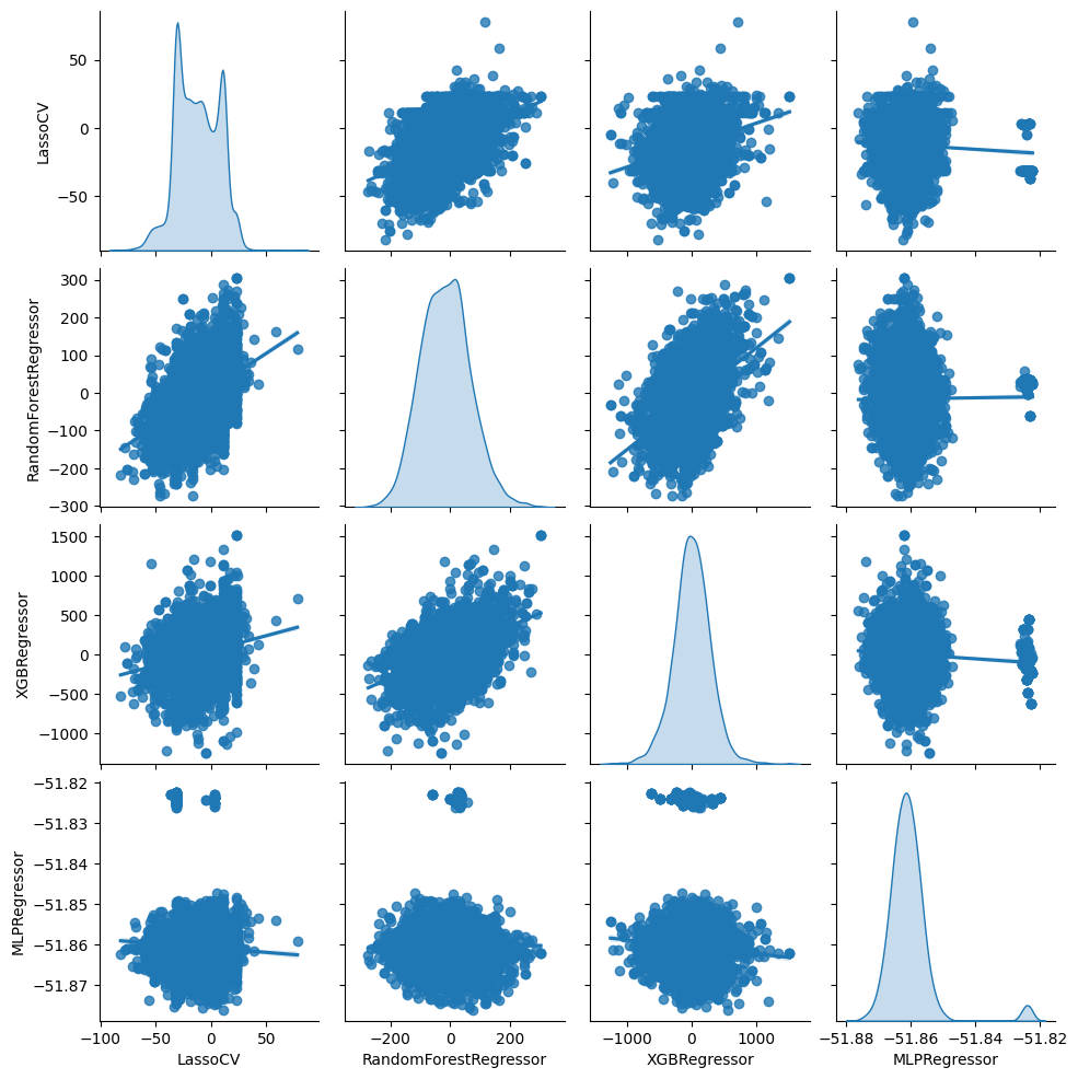
From the second table above, we see that regardless of the machine learning method, the estimated intercept (the first row of the table) is near 0 and statistically insignificant. Given our results for the unconditional ATE above, we should expect this. The estimate of the slopes are also either near 0, very imprecise, or both. This means that either the conditional average treatment effect is near 0 or that all four machine learning methods are very poor proxies for the true conditional average treatment effect.
Assisted Delivery#
Let’s see what we get when we look at assisted delivery.
ad = df.loc[X.index, "good_assisted_delivery"]#"midwife_birth"]
results_ad = evaluate_models(models, y=ad)
generate_report(results_ad)
Correlation in median CATE:
| LassoCV | RandomForestRegressor | XGBRegressor | MLPRegressor | |
|---|---|---|---|---|
| LassoCV | 1.000000 | 0.852487 | 0.506082 | 0.887314 |
| RandomForestRegressor | 0.852487 | 1.000000 | 0.580992 | 0.694986 |
| XGBRegressor | 0.506082 | 0.580992 | 1.000000 | 0.432495 |
| MLPRegressor | 0.887314 | 0.694986 | 0.432495 | 1.000000 |
Best linear projection of CATE
/tmp/ipykernel_2497/3641282101.py:16: FutureWarning: The previous implementation of stack is deprecated and will be removed in a future version of pandas. See the What's New notes for pandas 2.1.0 for details. Specify future_stack=True to adopt the new implementation and silence this warning.
  }).T.stack()
| LassoCV | RandomForestRegressor | XGBRegressor | MLPRegressor | ||
|---|---|---|---|---|---|
| blp | 0 | 0.049222 | 0.041678 | 0.037855 | 0.037895 |
| 1 | 0.387351 | 0.492484 | 0.136333 | 0.468474 | |
| se | 0 | 0.021575 | 0.022633 | 0.022036 | 0.021420 |
| 1 | 0.137844 | 0.152019 | 0.076830 | 0.126685 |
Group average treatment effects:
/tmp/ipykernel_2497/3641282101.py:23: FutureWarning: The previous implementation of stack is deprecated and will be removed in a future version of pandas. See the What's New notes for pandas 2.1.0 for details. Specify future_stack=True to adopt the new implementation and silence this warning.
  }).T.stack()
| LassoCV | RandomForestRegressor | XGBRegressor | MLPRegressor | ||
|---|---|---|---|---|---|
| gate | 0 | -0.020946 | -0.041124 | 0.011614 | 0.000063 |
| 1 | -0.011596 | -0.043113 | -0.010521 | -0.025810 | |
| 2 | 0.001884 | 0.025537 | 0.041182 | -0.027350 | |
| 3 | 0.096366 | 0.051628 | 0.066136 | 0.038021 | |
| 4 | 0.158910 | 0.199432 | 0.110033 | 0.204077 | |
| se | 0 | 0.035973 | 0.049924 | 0.051215 | 0.031466 |
| 1 | 0.045190 | 0.049240 | 0.047517 | 0.039677 | |
| 2 | 0.046322 | 0.040677 | 0.041650 | 0.049273 | |
| 3 | 0.046588 | 0.046432 | 0.045221 | 0.049899 | |
| 4 | 0.056614 | 0.051983 | 0.049597 | 0.057138 |
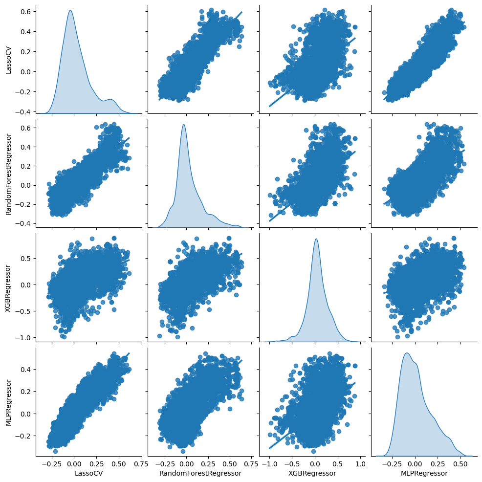
Now, the results are more encouraging. For all four machine learning methods, the slope estimate is positive and statistically significant. From this, we can conclude that the true conditional average treatment effect must vary with at least some covariates, and the machine learning proxies are at least somewhat correlated with the true conditional average treatment effect.
Covariate Means by Group#
Once we’ve detected heterogeneity in the grouped average treatment effects of using medical professionals for assisted delivery, it’s interesting to see how effects vary across groups. This could help us understand why the treatment effect varies or how to develop simple rules for targeting future treatments.
df2 = df.loc[X.index, :]
df2["edu99"] = df2.edu == 99
df2["educ"] = df2["edu"]
df2.loc[df2["edu99"], "educ"] = np.nan

variables = [
    "log_xp_percap","agecat","educ","tv","goat",
    "cow","motorbike","hh_cook_wood","pkh_ever"
]
def cov_mean_by_group(y, res, cluster_id):
    n_group = res["gate"].shape[1]
    gate = res["gate"].copy()
    gate_se = gate.copy()
    dat = y.to_frame()

    for i in range(res["cate"].shape[1]):
        S = res["cate"][:, i]
        cutoffs = np.quantile(S, np.linspace(0, 1, n_group+1))
        cutoffs[-1] += 1
        for k in range(n_group):
            dat[f"G{k}"] = ((cutoffs[k] <= S) & (S < cutoffs[k+1])) * 1.0

        g_form = "y ~ -1 + " + " + ".join([f"G{k}" for k in range(n_group)])
        g_reg = smf.ols(g_form, data=dat.astype(float))
        g_fit = g_reg.fit()
        gate[i, :] = g_fit.params.filter(regex="G").values
        rows = ~y.isna()
        gate_se[i, :] = get_treatment_se(g_fit, cluster_id, rows)

    out = pd.DataFrame(dict(
        mean=np.nanmedian(gate, axis=0),
        se=np.nanmedian(gate_se, axis=0),
        group=list(range(n_group))
    ))

    return out
def compute_group_means_for_results(results):
    to_cat = []
    for res in results:
        for v in variables:
            to_cat.append(
                cov_mean_by_group(df2[v], res, loc_id)
                .assign(method=res["name"], variable=v)
            )

    group_means = pd.concat(to_cat, ignore_index=True)
    group_means["plus2sd"] = group_means.eval("mean + 1.96*se")
    group_means["minus2sd"] = group_means.eval("mean - 1.96*se")
    return group_means
group_means_ad = compute_group_means_for_results(results_ad)
g = sns.FacetGrid(group_means_ad, col="variable", col_wrap=3, hue="method", sharey=False)
g.map(plt.plot, "group", "mean")
g.map(plt.plot, "group", "plus2sd", ls="--")
g.map(plt.plot, "group", "minus2sd", ls="--")
g.add_legend();
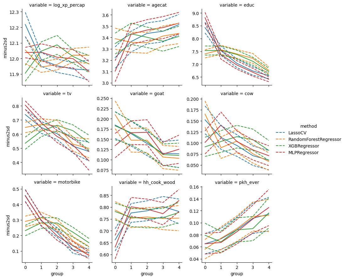
From this, we see that the group predicted to be most affected by treatment are less educated, less likely to own a TV or motorbike, and more likely to participate in the program.
If we wanted to maximize the program impact with a limited budget, targeting the program towards less educated and less wealthy mothers could be a good idea. The existing financial incentive already does this to some extent. As one might expect, a fixed-size cash incentive has a bigger behavioral impact on less wealthy individuals. If we want to further target these individuals, we could alter eligibility rules and/or increase the cash transfer for those with lower wealth.
Caution#
When exploring treatment heterogeneity like above, we need to interpret our results carefully. In particular, looking at grouped treatment effects and covariate means conditional on group leads to many hypothesis tests (although we never stated null hypotheses or reported p-values, the inevitable eye-balling of differences in the above graphs compared to their confidence intervals has the same issues as formal hypothesis tests). When we perform many hypothesis tests, we will likely stumble upon some statistically significant differences by chance. Therefore, writing about a single large difference found in the above analysis as though it is our main finding would be misleading (and perhaps unethical). The correct thing to do is to present all results that we have looked at. See this excellent news article by statistician Andrew Gelman for more information.
Causal Trees and Forests#
[hetAI16] develop the idea of “causal trees.” The purpose and method are qualitatively similar to the grouped average treatment effects. The main difference is that the groups in [hetAI16] are determined by a low-depth regression tree instead of by quantiles of a noisy estimate of the conditional average treatment effect. As above, sample-splitting is used to facilitate inference.
Causal trees share many downsides of regression trees. In particular, the branches of the tree and subsequent results can be sensitive to small changes in the data. [hetWA18] develop a causal forest estimator to address this concern. This causal forest estimates \(E[y_i(1) - y_i(0) |X_i=x]\) directly. Unlike most machine learning estimators, [hetWA18] prove that causal forests are consistent and pointwise asymptotically normal, albeit with a slower than \(\sqrt{n}\) rate of convergence. In practice, this means that either the sample size must be very large (and/or \(x\) relatively low dimension) to get precise estimates.
References#
- hetACE+11
Vivi Alatas, Nur Cahyadi, Elisabeth Ekasari, Sarah Harmoun, Budi Hidayat, Edgar Janz, Jon Jellema, H Tuhiman, and M Wai-Poi. Program keluarga harapan : impact evaluation of indonesia's pilot household conditional cash transfer program. Technical Report, World Bank, 2011. URL: http://documents.worldbank.org/curated/en/589171468266179965/Program-Keluarga-Harapan-impact-evaluation-of-Indonesias-Pilot-Household-Conditional-Cash-Transfer-Program.
- hetAI16(1,2,3)
Susan Athey and Guido Imbens. Recursive partitioning for heterogeneous causal effects. Proceedings of the National Academy of Sciences, 113(27):7353–7360, 2016. URL: http://www.pnas.org/content/113/27/7353, arXiv:http://www.pnas.org/content/113/27/7353.full.pdf, doi:10.1073/pnas.1510489113.
- hetCDDFV18(1,2,3)
Victor Chernozhukov, Mert Demirer, Esther Duflo, and Iván Fernández-Val. Generic machine learning inference on heterogenous treatment effects in randomized experimentsxo. Working Paper 24678, National Bureau of Economic Research, June 2018. URL: http://www.nber.org/papers/w24678, doi:10.3386/w24678.
- hetTri16(1,2)
Margaret Triyana. Do health care providers respond to demand-side incentives? evidence from indonesia. American Economic Journal: Economic Policy, 8(4):255–88, November 2016. URL: http://www.aeaweb.org/articles?id=10.1257/pol.20140048, doi:10.1257/pol.20140048.
- hetWA18(1,2,3)
Stefan Wager and Susan Athey. Estimation and inference of heterogeneous treatment effects using random forests. Journal of the American Statistical Association, 0(0):1–15, 2018. URL: https://doi.org/10.1080/01621459.2017.1319839, arXiv:https://doi.org/10.1080/01621459.2017.1319839, doi:10.1080/01621459.2017.1319839.