Getting Started#
Prerequisites
Good attitude
Good work ethic
Outcomes
Understand what a programming language is.
Know why we chose Python
Know what the Jupyter Notebook is
Be able to start JupyterLab in the chosen environment (cloud or personal computer)
Be able to open a Jupyter notebook in JupyterLab
Know Jupyter Notebook basics: cell modes, editing/evaluating cells
Welcome#
Welcome to the start of your path to learning how to work with data in the Python programming language!
A programming language is, loosely speaking, a structured subset of natural
language (words) and special characters (e.g. , or {) that allow humans
to describe operations they would like their computer to perform on their behalf.
The programming language translates these words and symbols into instructions the computer can execute.
Why Python?#
Among the hundreds of programming languages to choose from, we chose to teach you Python for the following reasons:
Easy to learn and use (relative to other programming languages).
Designed with readability in mind.
Excellent tools for handling data efficiently and succinctly.
Cemented as the world’s third most popular programming language, the most popular scripting language, and an increasing standard for data analysis in industry.
General purpose: Initially you will learn Python for data analysis, but it can also used for websites, database management, web scraping, financial modeling, data visualization, etc. In particular, it is the world’s best language for gluing those different pieces together.
However, the general purpose nature of Python comes at a cost: it is often said that Python is “the best language for nothing but the second best language for everything”.
We aren’t sure this is true, but a more optimistic view of that quote is that Python is a great language to have in your toolbox to solve all sorts of problems and patch them together.
A versatile “second-best” language might be the best one to learn first.
Some other languages to consider:
R has an impressive ecosystem of statistical packages, and is defensible as a choice for pure data science. It could be a useful second language to learn for projects that are entirely statistical.
Matlab has much more natural notation for writing linear algebra heavy code. However, it is: (a) expensive; (b) poor at dealing with data analysis; (c) grossly inferior to Python as a language; and (d) being left behind as Python and Julia ecosystems expand to more packages.
Julia is in part a far better version of Matlab, which can be as fast as Fortran or C. However, it has a young and immature environment and is currently more appropriate for academics and scientific computing specialists.
Another consideration for programming language choice is runtime performance. On this dimension, Python, R, and Matlab can be slow for certain types of tasks.
Luckily, this will not be an issue for data science and the types of analysis we will do in this course, because most of the data analytics packages in Python (and R) rely on high-performance code written in other languages in the background.
If you are writing more traditional scientific/technical computing in Python, there are things that can help make Python faster in some situations, but another language like Julia may be a better fit.
Why Open Source?#
Software development has changed radically in the last decade, increasingly becoming a process of stitching together both established high quality libraries, and state-of-the-art research projects.
A major disadvantage of Matlab, Stata, and other proprietary languages is that they are not open-source, and unable to work within this new paradigm.
Forgetting the cost for a moment, the benefits of using an open-source language are pragmatic rather than ideological.
Open source languages are easier for everyone in the world to write and share packages because the code is accessible and available.
With the right kinds of open source licenses; academics, businesses, and hobbyists all have incentives to contribute.
Because open-source languages are managed on publicly accessible sites (e.g. GitHub), it is easier to build a community and collaborate.
Package management systems (i.e. a way to find, download, install, and upgrade packages) in open-source languages can be very open and accessible since they don’t need to deal with proprietary software licenses.
Computing Environment#
These materials are meant to be interacted with, not passively read.
To help you do this, we use a software called Jupyter and files known as Jupyter notebooks which allow us to bundle a mixture of text, code, and code output together.
In fact, right now you are either directly reading a Jupyter notebook or a website that was generated from a Jupyter notebook.
Jupyter#
We will refer to two components of Jupyter’s software: JupyterLab and Jupyter Notebook.
JupyterLab
JupyterLab is a software that runs in your browser and allows you to do a variety of things such as: edit text, view files, and (most importantly) work with Jupyter notebooks.
Jupyter Notebook
This is the actual file that allows you to mix code and text.
The content inside a Jupyter notebook is organized into cells.
Cells can have inputs and outputs.
There are two main types of cells:
Markdown cells
Inputs are written in markdown and can contain formatted text, images, equations, and more.
Outputs are rendered in place of the input when the cell is executed.
Code cells
Inputs Contain Python code (or code in another language).
Outputs are placed below the input cell and contain the results generated when the input code is executed.
Below is an image that demonstrates what a Jupyter Notebook looks like:
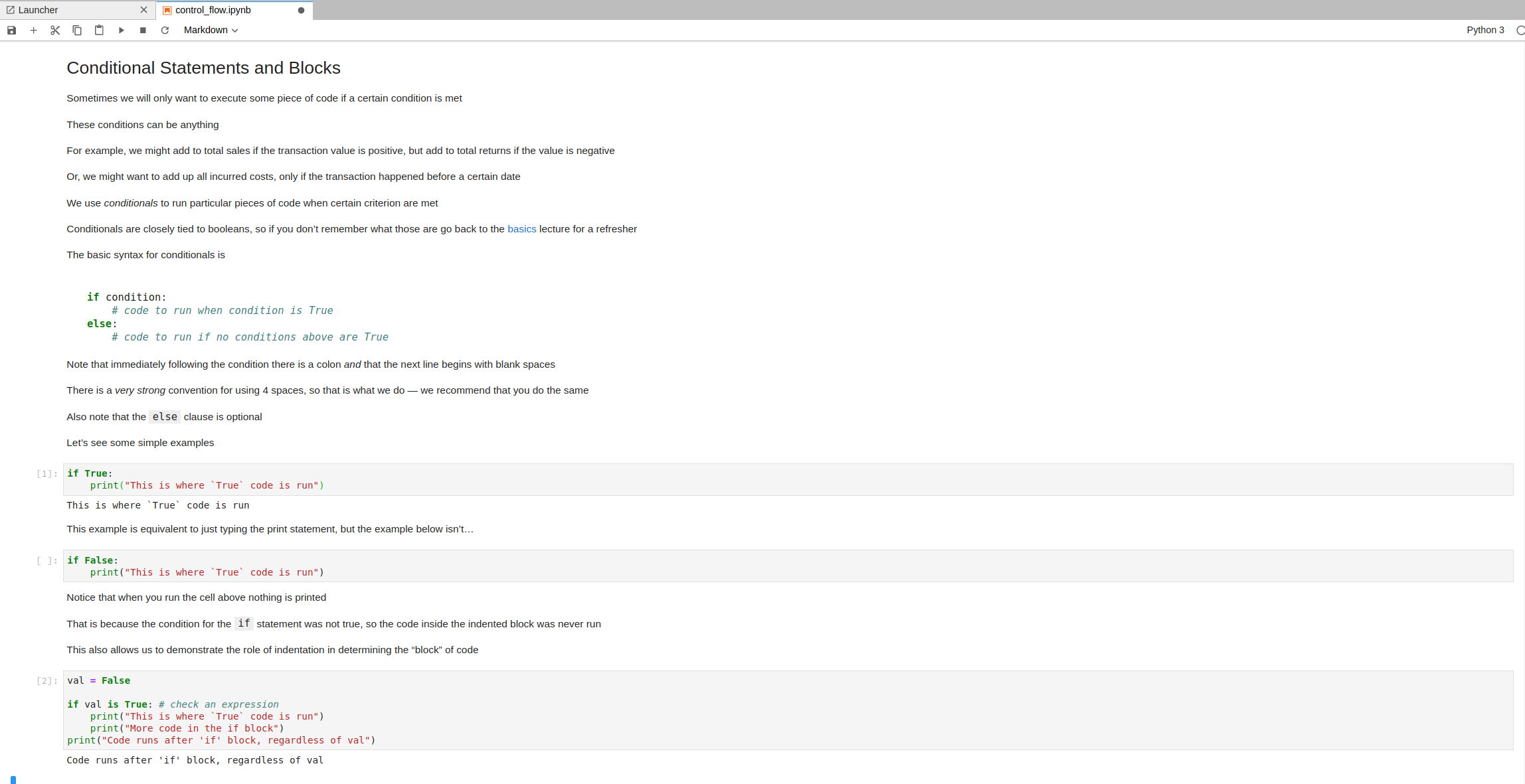
Notice a few things about this image:
Inputs to code cells have a
[ ]:to the left of them and have a darker background than the surrounding area.Code cells that have not yet been executed do not have a number in the
[ ]:box and have no corresponding output.Executed code cells have a
[#]:to the left of them (where#is a number) and, depending on what the code in that cell does, may or may not have an output.Executed markdown cells are displayed as formatted text, rather than the input/output structure.
Being able to include both text and code allows us to do interesting computations and explain them.
This combination has caused leading companies like Netflix and Bloomberg to adopt Jupyter as a tool of choice for data analytics and reporting.
We will follow in their path and leverage Jupyter Notebook throughout these materials.
Running the Lectures#
The interactivity of a Jupyter notebook is driven by two main components:
Server that is responsible for executing code
GUI that runs in your web browser (what we learned above above)
We will edit the content of the notebook and request code execution from the web GUI.
The Jupyter application will then ask the server to execute the code and send the results back to the GUI.
You can choose to interact with these materials from two server environments:
The cloud
Your own computer
Cloud Computing
A cloud solution provides a pre-installed environment for you.
As long as you have an internet connection, you will be able to interact with the lectures through a few cloud computing options.
We try to ensure that you’ll be able to run any of the lectures from each of the cloud options, but because these services are hosted by others, we cannot provide any guarantees.
Using the cloud is a great option if
You aren’t sure whether you’d like to learn these skills and just want to test the lectures out without any additional commitment.
You are away from your typical work station and would like to spend a few minutes interacting with our lectures — we often take this route with our colleagues over coffee (or other conversation stimulants).
If you would like to work on these lectures from the cloud, please read the instructions for getting set up with cloud computing.
These instructions describe several of the possible computing environments that you can choose, discuss their pros and cons, and explain what JupyterHub is.
After reading the instructions, return to this page and proceed with the Jupyter Basics section.
Local Installation
With a local installation, you will install the required software onto your own computer.
This is typically a straightforward task and, once you have done this, you will be able to run the lecture code (and any other code you write for your own projects!) on your personal computer.
If you are confident that these are skills you would like to acquire and are willing to have the software installed on your computer, then this is a great option.
If you would like to work from a local installation, please read the instructions in local installation instructions page.
These instructions will walk you through the installation procedure, help with some basic setup, and show you how to open JupyterLab.
Once you have completed installing the software, return to this page and proceed with the Jupyter Basics section.
Jupyter Basics#
Now that you can open a JupyterLab instance on the cloud or on your own computer, we can talk about how you should use them.
Note, not all of this will apply if you are using the Google Colab cloud server since they are running a modified version of Jupyter. For more help on using Colab, see their help menu.
JupyterLab Dashboard
When you open a new session in Jupyter, you will be taken to the JupyterLab dashboard page.
This page shows the file system of the machine running the Jupyter server and allows you to navigate and open particular Jupyter Notebooks (or other types of files!).
The dashboard page is shown below.
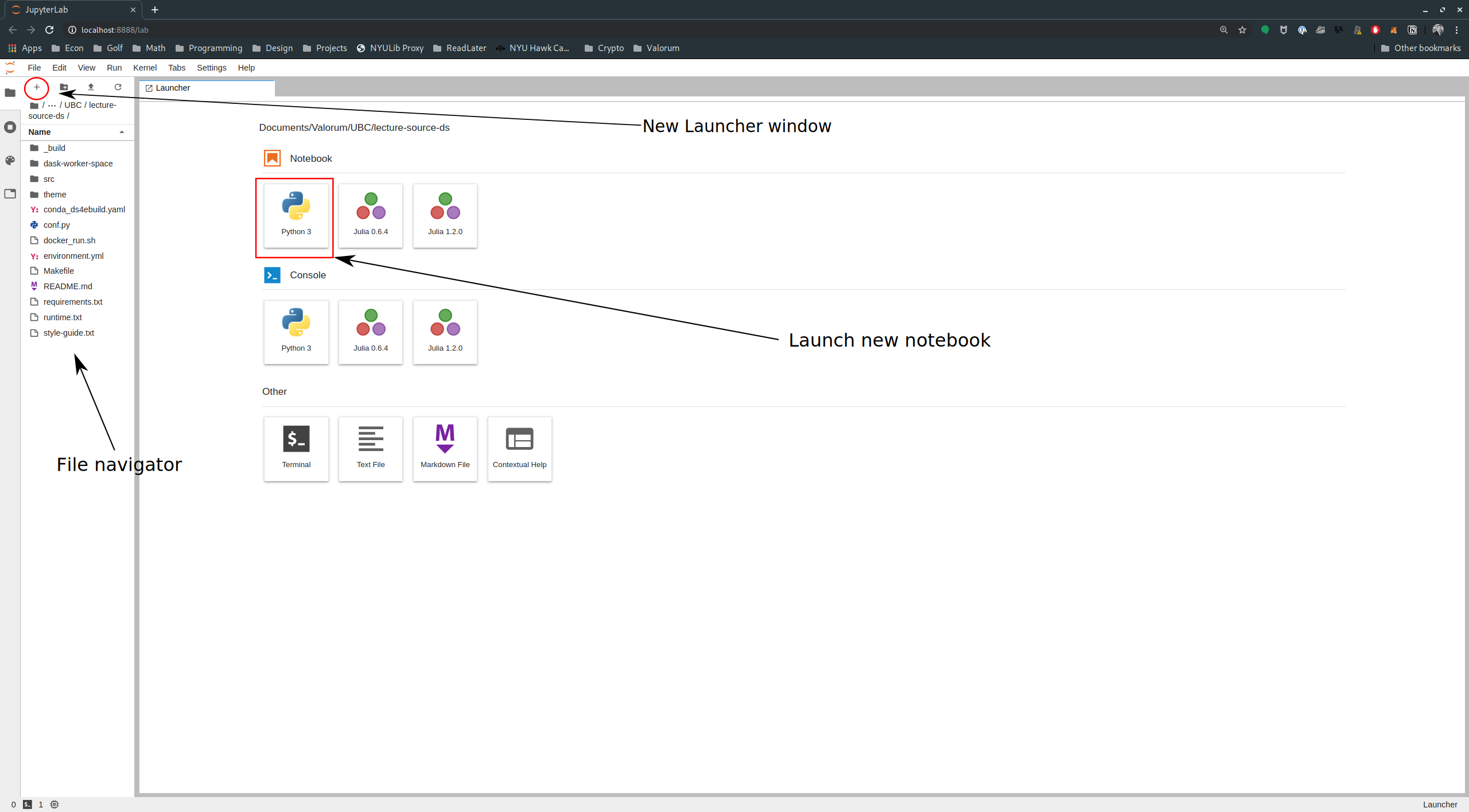
You can open existing files or change folders by double clicking on them in the left panel of the dashboard (similar to a file explorer you would find on your computer).
You can create new notebooks by clicking Python 3 in the Launcher (see red square in the image).
If you don’t see the Launcher as one of your tabs, you can open it by clicking the + at the top
of the file explorer section of the JupyterLab dashboard (see the red circle in the image).
Editing Jupyter Notebooks
Once you have opened a particular notebook, you can be in one of two “edit modes”.
Command mode: This mode is for making high level changes to the notebook itself. For example changing the order of cells, creating a new cell, etc…
You know you’re in command mode when a blue sidebar appears on the left of the cell.
Pressing keys tells Jupyter Notebook to run commands. For example,
aadds a new cell above the current cell,badds one below the current cell, anddddeletes the current cell.up arrow (or
k) changes the selected cell to the cell above the current one and down arrow (orj) changes to the cell below.
Edit mode: Used when editing the content inside of cells.
When in edit mode, the selected cell displays a green sidebar on left.
Can edit the content of a cell.
Some useful commands:
To go from command mode to edit mode, press enter or double click the mouse
Go from edit mode to command mode by pressing escape
You can evaluate a cell by pressing
Shift + Enter(meaningShiftandEnterat the same time)
Exercise
See exercise 1 in the exercise list.
Advanced Usage and Getting Help
For more help with JupyterLab and Jupyter Notebook, see the user guides:
Exercises#
Exercise 1#
In the code cell below (notice the [ ]: to the left) type a quote ("), your name,
then another quote (") and evaluate the cell
# code here!