Basic Functionality#
Prerequisites
Outcomes
Be familiar with
datetimeUse built-in aggregation functions and be able to create your own and apply them using
aggUse built-in Series transformation functions and be able to create your own and apply them using
applyUse built-in scalar transformation functions and be able to create your own and apply them using
mapBe able to select subsets of the DataFrame using boolean selection
Know what the “want operator” is and how to apply it
Data
US state unemployment data from Bureau of Labor Statistics
# Uncomment following line to install on colab
#! pip install
State Unemployment Data#
In this lecture, we will use unemployment data by state at a monthly frequency.
import pandas as pd

%matplotlib inline

pd.__version__
'2.2.3'
First, we will download the data directly from a url and read it into a pandas DataFrame.
## Load up the data -- this will take a couple seconds
url = "https://datascience.quantecon.org/assets/data/state_unemployment.csv"
unemp_raw = pd.read_csv(url, parse_dates=["Date"])
The pandas read_csv will determine most datatypes of the underlying columns. The
exception here is that we need to give pandas a hint so it can load up the Date column as a Python datetime type: the parse_dates=["Date"].
We can see the basic structure of the downloaded data by getting the first 5 rows, which directly matches the underlying CSV file.
unemp_raw.head()
| Date | state | LaborForce | UnemploymentRate | |
|---|---|---|---|---|
| 0 | 2000-01-01 | Alabama | 2142945.0 | 4.7 |
| 1 | 2000-01-01 | Alaska | 319059.0 | 6.3 |
| 2 | 2000-01-01 | Arizona | 2499980.0 | 4.1 |
| 3 | 2000-01-01 | Arkansas | 1264619.0 | 4.4 |
| 4 | 2000-01-01 | California | 16680246.0 | 5.0 |
Note that a row has a date, state, labor force size, and unemployment rate.
For our analysis, we want to look at the unemployment rate across different states over time, which requires a transformation of the data similar to an Excel pivot-table.
# Don't worry about the details here quite yet
unemp_all = (
    unemp_raw
    .reset_index()
    .pivot_table(index="Date", columns="state", values="UnemploymentRate")
)
unemp_all.head()
| state | Alabama | Alaska | Arizona | Arkansas | California | Colorado | Connecticut | Delaware | Florida | Georgia | ... | South Dakota | Tennessee | Texas | Utah | Vermont | Virginia | Washington | West Virginia | Wisconsin | Wyoming |
|---|---|---|---|---|---|---|---|---|---|---|---|---|---|---|---|---|---|---|---|---|---|
| Date | |||||||||||||||||||||
| 2000-01-01 | 4.7 | 6.3 | 4.1 | 4.4 | 5.0 | 2.8 | 2.8 | 3.5 | 3.7 | 3.7 | ... | 2.4 | 3.7 | 4.6 | 3.1 | 2.7 | 2.6 | 4.9 | 5.8 | 3.2 | 4.1 |
| 2000-02-01 | 4.7 | 6.3 | 4.1 | 4.3 | 5.0 | 2.8 | 2.7 | 3.6 | 3.7 | 3.6 | ... | 2.4 | 3.7 | 4.6 | 3.1 | 2.6 | 2.5 | 4.9 | 5.6 | 3.2 | 3.9 |
| 2000-03-01 | 4.6 | 6.3 | 4.0 | 4.3 | 5.0 | 2.7 | 2.6 | 3.6 | 3.7 | 3.6 | ... | 2.4 | 3.8 | 4.5 | 3.1 | 2.6 | 2.4 | 5.0 | 5.5 | 3.3 | 3.9 |
| 2000-04-01 | 4.6 | 6.3 | 4.0 | 4.3 | 5.1 | 2.7 | 2.5 | 3.7 | 3.7 | 3.7 | ... | 2.4 | 3.8 | 4.4 | 3.1 | 2.7 | 2.4 | 5.0 | 5.4 | 3.4 | 3.8 |
| 2000-05-01 | 4.5 | 6.3 | 4.0 | 4.2 | 5.1 | 2.7 | 2.4 | 3.7 | 3.7 | 3.7 | ... | 2.4 | 3.9 | 4.3 | 3.2 | 2.7 | 2.3 | 5.1 | 5.4 | 3.5 | 3.8 |
5 rows × 50 columns
Finally, we can filter it to look at a subset of the columns (i.e. “state” in this case).
states = [
    "Arizona", "California", "Florida", "Illinois",
    "Michigan", "New York", "Texas"
]
unemp = unemp_all[states]
unemp.head()
| state | Arizona | California | Florida | Illinois | Michigan | New York | Texas |
|---|---|---|---|---|---|---|---|
| Date | |||||||
| 2000-01-01 | 4.1 | 5.0 | 3.7 | 4.2 | 3.3 | 4.7 | 4.6 |
| 2000-02-01 | 4.1 | 5.0 | 3.7 | 4.2 | 3.2 | 4.7 | 4.6 |
| 2000-03-01 | 4.0 | 5.0 | 3.7 | 4.3 | 3.2 | 4.6 | 4.5 |
| 2000-04-01 | 4.0 | 5.1 | 3.7 | 4.3 | 3.3 | 4.6 | 4.4 |
| 2000-05-01 | 4.0 | 5.1 | 3.7 | 4.3 | 3.5 | 4.6 | 4.3 |
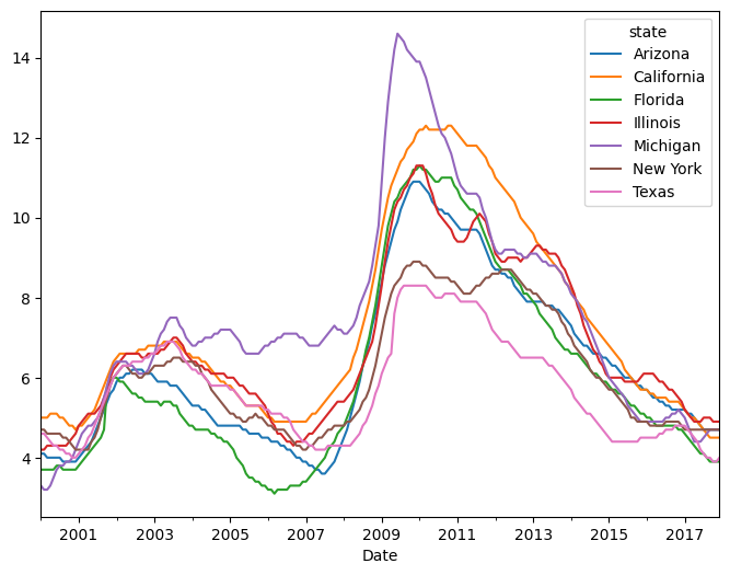
When plotting, a DataFrame knows the column and index names.
unemp.plot(figsize=(8, 6))
<Axes: xlabel='Date'>
Exercise
See exercise 1 in the exercise list.
Dates in pandas#
You might have noticed that our index now has a nice format for the
dates (YYYY-MM-DD) rather than just a year.
This is because the dtype of the index is a variant of datetime.
unemp.index
DatetimeIndex(['2000-01-01', '2000-02-01', '2000-03-01', '2000-04-01',
               '2000-05-01', '2000-06-01', '2000-07-01', '2000-08-01',
               '2000-09-01', '2000-10-01',
               ...
               '2017-03-01', '2017-04-01', '2017-05-01', '2017-06-01',
               '2017-07-01', '2017-08-01', '2017-09-01', '2017-10-01',
               '2017-11-01', '2017-12-01'],
              dtype='datetime64[ns]', name='Date', length=216, freq=None)
We can index into a DataFrame with a DatetimeIndex using string
representations of dates.
For example
# Data corresponding to a single date
unemp.loc["01/01/2000", :]
state
Arizona       4.1
California    5.0
Florida       3.7
Illinois      4.2
Michigan      3.3
New York      4.7
Texas         4.6
Name: 2000-01-01 00:00:00, dtype: float64
# Data for all days between New Years Day and June first in the year 2000
unemp.loc["01/01/2000":"06/01/2000", :]
| state | Arizona | California | Florida | Illinois | Michigan | New York | Texas |
|---|---|---|---|---|---|---|---|
| Date | |||||||
| 2000-01-01 | 4.1 | 5.0 | 3.7 | 4.2 | 3.3 | 4.7 | 4.6 |
| 2000-02-01 | 4.1 | 5.0 | 3.7 | 4.2 | 3.2 | 4.7 | 4.6 |
| 2000-03-01 | 4.0 | 5.0 | 3.7 | 4.3 | 3.2 | 4.6 | 4.5 |
| 2000-04-01 | 4.0 | 5.1 | 3.7 | 4.3 | 3.3 | 4.6 | 4.4 |
| 2000-05-01 | 4.0 | 5.1 | 3.7 | 4.3 | 3.5 | 4.6 | 4.3 |
| 2000-06-01 | 4.0 | 5.1 | 3.8 | 4.3 | 3.7 | 4.6 | 4.3 |
We will learn more about what pandas can do with dates and times in an upcoming lecture on time series data.
DataFrame Aggregations#
Let’s talk about aggregations.
Loosely speaking, an aggregation is an operation that combines multiple values into a single value.
For example, computing the mean of three numbers (for example
[0, 1, 2]) returns a single number (1).
We will use aggregations extensively as we analyze and manipulate our data.
Thankfully, pandas makes this easy!
Built-in Aggregations#
pandas already has some of the most frequently used aggregations.
For example:
Mean (
mean)Variance (
var)Standard deviation (
std)Minimum (
min)Median (
median)Maximum (
max)etc…
Note
When looking for common operations, using “tab completion” goes a long way.
unemp.mean()
state
Arizona       6.301389
California    7.299074
Florida       6.048611
Illinois      6.822685
Michigan      7.492593
New York      6.102315
Texas         5.695370
dtype: float64
As seen above, the aggregation’s default is to aggregate each column.
However, by using the axis keyword argument, you can do aggregations by
row as well.
unemp.var(axis=1).head()
Date
2000-01-01    0.352381
2000-02-01    0.384762
2000-03-01    0.364762
2000-04-01    0.353333
2000-05-01    0.294762
dtype: float64
Writing Your Own Aggregation#
The built-in aggregations will get us pretty far in our analysis, but sometimes we need more flexibility.
We can have pandas perform custom aggregations by following these two steps:
Write a Python function that takes a
Seriesas an input and outputs a single value.Call the
aggmethod with our new function as an argument.
For example, below, we will classify states as “low unemployment” or “high unemployment” based on whether their mean unemployment level is above or below 6.5.
#
# Step 1: We write the (aggregation) function that we'd like to use
#
def high_or_low(s):
    """
    This function takes a pandas Series object and returns high
    if the mean is above 6.5 and low if the mean is below 6.5
    """
    if s.mean() < 6.5:
        out = "Low"
    else:
        out = "High"

    return out
#
# Step 2: Apply it via the agg method.
#
unemp.agg(high_or_low)
state
Arizona        Low
California    High
Florida        Low
Illinois      High
Michigan      High
New York       Low
Texas          Low
dtype: object
# How does this differ from unemp.agg(high_or_low)?
unemp.agg(high_or_low, axis=1).head()
Date
2000-01-01    Low
2000-02-01    Low
2000-03-01    Low
2000-04-01    Low
2000-05-01    Low
dtype: object
Notice that agg can also accept multiple functions at once.
unemp.agg([min, max, high_or_low])
/tmp/ipykernel_2992/286408109.py:1: FutureWarning: The provided callable <built-in function min> is currently using Series.min. In a future version of pandas, the provided callable will be used directly. To keep current behavior pass the string "min" instead.
  unemp.agg([min, max, high_or_low])
/tmp/ipykernel_2992/286408109.py:1: FutureWarning: The provided callable <built-in function max> is currently using Series.max. In a future version of pandas, the provided callable will be used directly. To keep current behavior pass the string "max" instead.
  unemp.agg([min, max, high_or_low])
| state | Arizona | California | Florida | Illinois | Michigan | New York | Texas |
|---|---|---|---|---|---|---|---|
| min | 3.6 | 4.5 | 3.1 | 4.2 | 3.2 | 4.2 | 3.9 |
| max | 10.9 | 12.3 | 11.3 | 11.3 | 14.6 | 8.9 | 8.3 |
| high_or_low | Low | High | Low | High | High | Low | Low |
Exercise
See exercise 2 in the exercise list.
Transforms#
Many analytical operations do not necessarily involve an aggregation.
The output of a function applied to a Series might need to be a new Series.
Some examples:
Compute the percentage change in unemployment from month to month.
Calculate the cumulative sum of elements in each column.
Built-in Transforms#
pandas comes with many transform functions including:
Cumulative sum/max/min/product (
cum(sum|min|max|prod))Difference (
diff)Elementwise addition/subtraction/multiplication/division (
+,-,*,/)Percent change (
pct_change)Number of occurrences of each distinct value (
value_counts)Absolute value (
abs)
Again, tab completion is helpful when trying to find these functions.
unemp.head()
| state | Arizona | California | Florida | Illinois | Michigan | New York | Texas |
|---|---|---|---|---|---|---|---|
| Date | |||||||
| 2000-01-01 | 4.1 | 5.0 | 3.7 | 4.2 | 3.3 | 4.7 | 4.6 |
| 2000-02-01 | 4.1 | 5.0 | 3.7 | 4.2 | 3.2 | 4.7 | 4.6 |
| 2000-03-01 | 4.0 | 5.0 | 3.7 | 4.3 | 3.2 | 4.6 | 4.5 |
| 2000-04-01 | 4.0 | 5.1 | 3.7 | 4.3 | 3.3 | 4.6 | 4.4 |
| 2000-05-01 | 4.0 | 5.1 | 3.7 | 4.3 | 3.5 | 4.6 | 4.3 |
unemp.pct_change(fill_method = None).head() # Skip calculation for missing data
| state | Arizona | California | Florida | Illinois | Michigan | New York | Texas |
|---|---|---|---|---|---|---|---|
| Date | |||||||
| 2000-01-01 | NaN | NaN | NaN | NaN | NaN | NaN | NaN |
| 2000-02-01 | 0.00000 | 0.00 | 0.0 | 0.00000 | -0.030303 | 0.000000 | 0.000000 |
| 2000-03-01 | -0.02439 | 0.00 | 0.0 | 0.02381 | 0.000000 | -0.021277 | -0.021739 |
| 2000-04-01 | 0.00000 | 0.02 | 0.0 | 0.00000 | 0.031250 | 0.000000 | -0.022222 |
| 2000-05-01 | 0.00000 | 0.00 | 0.0 | 0.00000 | 0.060606 | 0.000000 | -0.022727 |
unemp.diff().head()
| state | Arizona | California | Florida | Illinois | Michigan | New York | Texas |
|---|---|---|---|---|---|---|---|
| Date | |||||||
| 2000-01-01 | NaN | NaN | NaN | NaN | NaN | NaN | NaN |
| 2000-02-01 | 0.0 | 0.0 | 0.0 | 0.0 | -0.1 | 0.0 | 0.0 |
| 2000-03-01 | -0.1 | 0.0 | 0.0 | 0.1 | 0.0 | -0.1 | -0.1 |
| 2000-04-01 | 0.0 | 0.1 | 0.0 | 0.0 | 0.1 | 0.0 | -0.1 |
| 2000-05-01 | 0.0 | 0.0 | 0.0 | 0.0 | 0.2 | 0.0 | -0.1 |
Transforms can be split into to several main categories:
Series transforms: functions that take in one Series and produce another Series. The index of the input and output does not need to be the same.
Scalar transforms: functions that take a single value and produce a single value. An example is the
absmethod, or adding a constant to each value of a Series.
Custom Series Transforms#
pandas also simplifies applying custom Series transforms to a Series or the columns of a DataFrame. The steps are:
Write a Python function that takes a Series and outputs a new Series.
Pass our new function as an argument to the
applymethod (alternatively, thetransformmethod).
As an example, we will standardize our unemployment data to have mean 0 and standard deviation 1.
After doing this, we can use an aggregation to determine at which date the unemployment rate is most different from “normal times” for each state.
#
# Step 1: We write the Series transform function that we'd like to use
#
def standardize_data(x):
    """
    Changes the data in a Series to become mean 0 with standard deviation 1
    """
    mu = x.mean()
    std = x.std()

    return (x - mu)/std
#
# Step 2: Apply our function via the apply method.
#
std_unemp = unemp.apply(standardize_data)
std_unemp.head()
| state | Arizona | California | Florida | Illinois | Michigan | New York | Texas |
|---|---|---|---|---|---|---|---|
| Date | |||||||
| 2000-01-01 | -1.076861 | -0.935545 | -0.976846 | -1.337203 | -1.605740 | -0.925962 | -0.849345 |
| 2000-02-01 | -1.076861 | -0.935545 | -0.976846 | -1.337203 | -1.644039 | -0.925962 | -0.849345 |
| 2000-03-01 | -1.125778 | -0.935545 | -0.976846 | -1.286217 | -1.644039 | -0.991993 | -0.926885 |
| 2000-04-01 | -1.125778 | -0.894853 | -0.976846 | -1.286217 | -1.605740 | -0.991993 | -1.004424 |
| 2000-05-01 | -1.125778 | -0.894853 | -0.976846 | -1.286217 | -1.529141 | -0.991993 | -1.081964 |
# Takes the absolute value of all elements of a function
abs_std_unemp = std_unemp.abs()

abs_std_unemp.head()
| state | Arizona | California | Florida | Illinois | Michigan | New York | Texas |
|---|---|---|---|---|---|---|---|
| Date | |||||||
| 2000-01-01 | 1.076861 | 0.935545 | 0.976846 | 1.337203 | 1.605740 | 0.925962 | 0.849345 |
| 2000-02-01 | 1.076861 | 0.935545 | 0.976846 | 1.337203 | 1.644039 | 0.925962 | 0.849345 |
| 2000-03-01 | 1.125778 | 0.935545 | 0.976846 | 1.286217 | 1.644039 | 0.991993 | 0.926885 |
| 2000-04-01 | 1.125778 | 0.894853 | 0.976846 | 1.286217 | 1.605740 | 0.991993 | 1.004424 |
| 2000-05-01 | 1.125778 | 0.894853 | 0.976846 | 1.286217 | 1.529141 | 0.991993 | 1.081964 |
# find the date when unemployment was "most different from normal" for each State
def idxmax(x):
    # idxmax of Series will return index of maximal value
    return x.idxmax()

abs_std_unemp.agg(idxmax)
state
Arizona      2009-11-01
California   2010-03-01
Florida      2010-01-01
Illinois     2009-12-01
Michigan     2009-06-01
New York     2009-11-01
Texas        2009-08-01
dtype: datetime64[ns]
Custom Scalar Transforms#
As you may have predicted, we can also apply custom scalar transforms to our pandas data.
To do this, we use the following pattern:
Define a Python function that takes in a scalar and produces a scalar.
Pass this function as an argument to the
mapSeries or DataFrame method.
Complete the exercise below to practice writing and using your own scalar transforms.
Exercise
See exercise 3 in the exercise list.
Boolean Selection#
We have seen how we can select subsets of data by referring to the index or column names.
However, we often want to select based on conditions met by the data itself.
Some examples are:
Restrict analysis to all individuals older than 18.
Look at data that corresponds to particular time periods.
Analyze only data that corresponds to a recession.
Obtain data for a specific product or customer ID.
We will be able to do this by using a Series or list of boolean values to index into a Series or DataFrame.
Let’s look at some examples.
unemp_small = unemp.head()  # Create smaller data so we can see what's happening
unemp_small
| state | Arizona | California | Florida | Illinois | Michigan | New York | Texas |
|---|---|---|---|---|---|---|---|
| Date | |||||||
| 2000-01-01 | 4.1 | 5.0 | 3.7 | 4.2 | 3.3 | 4.7 | 4.6 |
| 2000-02-01 | 4.1 | 5.0 | 3.7 | 4.2 | 3.2 | 4.7 | 4.6 |
| 2000-03-01 | 4.0 | 5.0 | 3.7 | 4.3 | 3.2 | 4.6 | 4.5 |
| 2000-04-01 | 4.0 | 5.1 | 3.7 | 4.3 | 3.3 | 4.6 | 4.4 |
| 2000-05-01 | 4.0 | 5.1 | 3.7 | 4.3 | 3.5 | 4.6 | 4.3 |
# list of booleans selects rows
unemp_small.loc[[True, True, True, False, False]]
| state | Arizona | California | Florida | Illinois | Michigan | New York | Texas |
|---|---|---|---|---|---|---|---|
| Date | |||||||
| 2000-01-01 | 4.1 | 5.0 | 3.7 | 4.2 | 3.3 | 4.7 | 4.6 |
| 2000-02-01 | 4.1 | 5.0 | 3.7 | 4.2 | 3.2 | 4.7 | 4.6 |
| 2000-03-01 | 4.0 | 5.0 | 3.7 | 4.3 | 3.2 | 4.6 | 4.5 |
# second argument selects columns, the  ``:``  means "all".
# here we use it to select all columns
unemp_small.loc[[True, False, True, False, True], :]
| state | Arizona | California | Florida | Illinois | Michigan | New York | Texas |
|---|---|---|---|---|---|---|---|
| Date | |||||||
| 2000-01-01 | 4.1 | 5.0 | 3.7 | 4.2 | 3.3 | 4.7 | 4.6 |
| 2000-03-01 | 4.0 | 5.0 | 3.7 | 4.3 | 3.2 | 4.6 | 4.5 |
| 2000-05-01 | 4.0 | 5.1 | 3.7 | 4.3 | 3.5 | 4.6 | 4.3 |
# can use booleans to select both rows and columns
unemp_small.loc[[True, True, True, False, False], [True, False, False, False, False, True, True]]
| state | Arizona | New York | Texas |
|---|---|---|---|
| Date | |||
| 2000-01-01 | 4.1 | 4.7 | 4.6 |
| 2000-02-01 | 4.1 | 4.7 | 4.6 |
| 2000-03-01 | 4.0 | 4.6 | 4.5 |
Creating Boolean DataFrames/Series#
We can use conditional statements to construct Series of booleans from our data.
unemp_small["Texas"] < 4.5
Date
2000-01-01    False
2000-02-01    False
2000-03-01    False
2000-04-01     True
2000-05-01     True
Name: Texas, dtype: bool
Once we have our Series of bools, we can use it to extract subsets of rows from our DataFrame.
unemp_small.loc[unemp_small["Texas"] < 4.5]
| state | Arizona | California | Florida | Illinois | Michigan | New York | Texas |
|---|---|---|---|---|---|---|---|
| Date | |||||||
| 2000-04-01 | 4.0 | 5.1 | 3.7 | 4.3 | 3.3 | 4.6 | 4.4 |
| 2000-05-01 | 4.0 | 5.1 | 3.7 | 4.3 | 3.5 | 4.6 | 4.3 |
unemp_small["New York"] > unemp_small["Texas"]
Date
2000-01-01    True
2000-02-01    True
2000-03-01    True
2000-04-01    True
2000-05-01    True
dtype: bool
big_NY = unemp_small["New York"] > unemp_small["Texas"]
unemp_small.loc[big_NY]
| state | Arizona | California | Florida | Illinois | Michigan | New York | Texas |
|---|---|---|---|---|---|---|---|
| Date | |||||||
| 2000-01-01 | 4.1 | 5.0 | 3.7 | 4.2 | 3.3 | 4.7 | 4.6 |
| 2000-02-01 | 4.1 | 5.0 | 3.7 | 4.2 | 3.2 | 4.7 | 4.6 |
| 2000-03-01 | 4.0 | 5.0 | 3.7 | 4.3 | 3.2 | 4.6 | 4.5 |
| 2000-04-01 | 4.0 | 5.1 | 3.7 | 4.3 | 3.3 | 4.6 | 4.4 |
| 2000-05-01 | 4.0 | 5.1 | 3.7 | 4.3 | 3.5 | 4.6 | 4.3 |
Multiple Conditions#
In the boolean section of the basics lecture, we saw
that we can use the words and and or to combine multiple booleans into
a single bool.
Recall:
True and False -> FalseTrue and True -> TrueFalse and False -> FalseTrue or False -> TrueTrue or True -> TrueFalse or False -> False
We can do something similar in pandas, but instead of
bool1 and bool2 we write:
(bool_series1) & (bool_series2)
Likewise, instead of bool1 or bool2 we write:
(bool_series1) | (bool_series2)
small_NYTX = (unemp_small["Texas"] < 4.7) & (unemp_small["New York"] < 4.7)
small_NYTX
Date
2000-01-01    False
2000-02-01    False
2000-03-01     True
2000-04-01     True
2000-05-01     True
dtype: bool
unemp_small[small_NYTX]
| state | Arizona | California | Florida | Illinois | Michigan | New York | Texas |
|---|---|---|---|---|---|---|---|
| Date | |||||||
| 2000-03-01 | 4.0 | 5.0 | 3.7 | 4.3 | 3.2 | 4.6 | 4.5 |
| 2000-04-01 | 4.0 | 5.1 | 3.7 | 4.3 | 3.3 | 4.6 | 4.4 |
| 2000-05-01 | 4.0 | 5.1 | 3.7 | 4.3 | 3.5 | 4.6 | 4.3 |
isin#
Sometimes, we will want to check whether a data point takes on one of a several fixed values.
We could do this by writing (df["x"] == val_1) | (df["x"] == val_2)
(like we did above), but there is a better way: the .isin method
unemp_small["Michigan"].isin([3.3, 3.2])
Date
2000-01-01     True
2000-02-01     True
2000-03-01     True
2000-04-01     True
2000-05-01    False
Name: Michigan, dtype: bool
# now select full rows where this Series is True
unemp_small.loc[unemp_small["Michigan"].isin([3.3, 3.2])]
| state | Arizona | California | Florida | Illinois | Michigan | New York | Texas |
|---|---|---|---|---|---|---|---|
| Date | |||||||
| 2000-01-01 | 4.1 | 5.0 | 3.7 | 4.2 | 3.3 | 4.7 | 4.6 |
| 2000-02-01 | 4.1 | 5.0 | 3.7 | 4.2 | 3.2 | 4.7 | 4.6 |
| 2000-03-01 | 4.0 | 5.0 | 3.7 | 4.3 | 3.2 | 4.6 | 4.5 |
| 2000-04-01 | 4.0 | 5.1 | 3.7 | 4.3 | 3.3 | 4.6 | 4.4 |
.any and .all#
Recall from the boolean section of the basics lecture
that the Python functions any and all are aggregation functions that
take a collection of booleans and return a single boolean.
any returns True whenever at least one of the inputs are True while
all is True only when all the inputs are True.
Series and DataFrames with dtype bool have .any and .all
methods that apply this logic to pandas objects.
Let’s use these methods to count how many months all the states in our sample had high unemployment.
As we work through this example, consider the “want operator”, a helpful concept from Nobel Laureate Tom Sargent for clearly stating the goal of our analysis and determining the steps necessary to reach the goal.
We always begin by writing Want: followed by what we want to
accomplish.
In this case, we would write:
Want: Count the number of months in which all states in our sample had unemployment above 6.5%
After identifying the want, we work backwards to identify the steps necessary to accomplish our goal.
So, starting from the result, we have:
Sum the number of
Truevalues in a Series indicating dates for which all states had high unemployment.Build the Series used in the last step by using the
.allmethod on a DataFrame containing booleans indicating whether each state had high unemployment at each date.Build the DataFrame used in the previous step using a
>comparison.
Now that we have a clear plan, let’s follow through and apply the want operator:
# Step 3: construct the DataFrame of bools
high = unemp > 6.5
high.head()
| state | Arizona | California | Florida | Illinois | Michigan | New York | Texas |
|---|---|---|---|---|---|---|---|
| Date | |||||||
| 2000-01-01 | False | False | False | False | False | False | False |
| 2000-02-01 | False | False | False | False | False | False | False |
| 2000-03-01 | False | False | False | False | False | False | False |
| 2000-04-01 | False | False | False | False | False | False | False |
| 2000-05-01 | False | False | False | False | False | False | False |
# Step 2: use the .all method on axis=1 to get the dates where all states have a True
all_high = high.all(axis=1)
all_high.head()
Date
2000-01-01    False
2000-02-01    False
2000-03-01    False
2000-04-01    False
2000-05-01    False
dtype: bool
# Step 1: Call .sum to add up the number of True values in `all_high`
#         (note that True == 1 and False == 0 in Python, so .sum will count Trues)
msg = "Out of {} months, {} had high unemployment across all states"
print(msg.format(len(all_high), all_high.sum()))
Out of 216 months, 41 had high unemployment across all states
Exercise
See exercise 4 in the exercise list.
Exercises#
Exercise 1#
Looking at the displayed DataFrame above, can you identify the index? The columns?
You can use the cell below to verify your visual intuition.
# your code here
Exercise 2#
Do the following exercises in separate code cells below:
At each date, what is the minimum unemployment rate across all states in our sample?
What was the median unemployment rate in each state?
What was the maximum unemployment rate across the states in our sample? What state did it happen in? In what month/year was this achieved?
Hint
What Python type (not
dtype) is returned by the aggregation?Hint
Read documentation for the method
idxmax.
Classify each state as high or low volatility based on whether the variance of their unemployment is above or below 4.
# min unemployment rate by state
# median unemployment rate by state
# max unemployment rate across all states and Year
# low or high volatility
Exercise 3#
Imagine that we want to determine whether unemployment was high (> 6.5), medium (4.5 < x <= 6.5), or low (<= 4.5) for each state and each month.
Write a Python function that takes a single number as an input and outputs a single string noting if that number is high, medium, or low.
Pass your function to
map(quiz: whymapand notaggorapply?) and save the result in a new DataFrame calledunemp_bins.(Challenging) This exercise has multiple parts:
Use another transform on
unemp_binsto count how many times each state had each of the three classifications.Hint
Will this value counting function be a Series or scalar transform?
Hint
Try googling “pandas count unique value” or something similar to find the right transform.
Construct a horizontal bar chart of the number of occurrences of each level with one bar per state and classification (21 total bars).
(Challenging) Repeat the previous step, but count how many states had each classification in each month. Which month had the most states with high unemployment? What about medium and low?
# Part 1: Write a Python function to classify unemployment levels.
# Part 2: Pass your function from part 1 to map
unemp_bins = unemp.map#replace this comment with your code!!
# Part 3: Count the number of times each state had each classification.

## then make a horizontal bar chart here
# Part 4: Apply the same transform from part 4, but to each date instead of to each state.
Exercise 4#
For a single state of your choice, determine what the mean unemployment is during “Low”, “Medium”, and “High” unemployment times (recall your
unemp_binsDataFrame from the exercise above).Think about how you would do this for all the states in our sample and write your thoughts… We will soon learn tools that will greatly simplify operations like this that operate on distinct groups of data at a time.
Which states in our sample performs the best during “bad times?” To determine this, compute the mean unemployment for each state only for months in which the mean unemployment rate in our sample is greater than 7.