Reshape

Prerequisites

• pandas intro

• pandas basics

• Importance of index

Outcomes

• Understand and be able to apply the melt/stack/unstack/pivot methods

• Practice transformations of indices

• Understand tidy data

# Uncomment following line to install on colab
#! pip install 

import numpy as np
import pandas as pd

%matplotlib inline

Tidy Data

While pushed more generally in the R language, the concept of “tidy data” is helpful in understanding the objectives for reshaping data, which in turn makes advanced features like groupby more seamless.

Hadley Wickham gives a terminology slightly better-adapted for the experimental sciences, but nevertheless useful for the social sciences.

A dataset is a collection of values, usually either numbers (if quantitative) or strings (if qualitative). Values are organized in two ways. Every value belongs to a variable and an observation. A variable contains all values that measure the same underlying attribute (like height, temperature, duration) across units. An observation contains all values measured on the same unit (like a person, or a day, or a race) across attributes. – Tidy Data (Journal of Statistical Software 2013)

With this framing,

A dataset is messy or tidy depending on how rows, columns and tables are matched with observations, variables, and types. In tidy data:

1. Each variable forms a column.

2. Each observation forms a row.

3. Each type of observational unit forms a table.

The “column” and “row” terms map directly to pandas columns and rows, while the “table” maps to a pandas DataFrame.

With this thinking and interpretation, it becomes essential to think through what uniquely identifies an “observation” in your data.

Is it a country? A year? A combination of country and year?

These will become the indices of your DataFrame.

For those with more of a database background, the “tidy” format matches the 3rd normal form in database theory, where the referential integrity of the database is maintained by the uniqueness of the index.

When considering how to map this to the social sciences, note that reshaping data can change what we consider to be the variable and observation in a way that doesn’t occur within the natural sciences.

For example, if the “observation” uniquely identified by a country and year and the “variable” is GDP, you may wish to reshape it so that the “observable” is a country, and the variables are a GDP for each year.

A word of caution: The tidy approach, where there is no redundancy and each type of observational unit forms a table, is a good approach for storing data, but you will frequently reshape/merge/etc. in order to make graphing or analysis easier. This doesn’t break the tidy format since those examples are ephemeral states used in analysis.

Reshaping your Data

The data you receive is not always in a “shape” that makes it easy to analyze.

What do we mean by shape? The number of rows and columns in a DataFrame and how information is stored in the index and column names.

This lecture will teach you the basic concepts of reshaping data.

As with other topics, we recommend reviewing the pandas documentation on this subject for additional information.

We will keep our discussion here as brief and simple as possible because these tools will reappear in subsequent lectures.

url = "https://datascience.quantecon.org/assets/data/bball.csv"
bball = pd.read_csv(url)
bball.info()

bball

<class 'pandas.core.frame.DataFrame'>
RangeIndex: 9 entries, 0 to 8
Data columns (total 8 columns):
 #   Column    Non-Null Count  Dtype  
---  ------    --------------  -----  
 0   Year      9 non-null      int64  
 1   Player    9 non-null      object 
 2   Team      9 non-null      object 
 3   TeamName  9 non-null      object 
 4   Games     9 non-null      int64  
 5   Pts       9 non-null      float64
 6   Assist    9 non-null      float64
 7   Rebound   9 non-null      float64
dtypes: float64(3), int64(2), object(3)
memory usage: 708.0+ bytes

	Year	Player	Team	TeamName	Games	Pts	Assist	Rebound
0	2015	Curry	GSW	Warriors	79	30.1	6.7	5.4
1	2016	Curry	GSW	Warriors	79	25.3	6.6	4.5
2	2017	Curry	GSW	Warriors	51	26.4	6.1	5.1
3	2015	Durant	OKC	Thunder	72	28.2	5.0	8.2
4	2016	Durant	GSW	Warriors	62	25.1	4.8	8.3
5	2017	Durant	GSW	Warriors	68	26.4	5.4	6.8
6	2015	Ibaka	OKC	Thunder	78	12.6	0.8	6.8
7	2016	Ibaka	ORL	Magic	56	15.1	1.1	6.8
8	2016	Ibaka	TOR	Raptors	23	14.2	0.7	6.8

Long vs Wide

Many of these operations change between long and wide DataFrames.

What does it mean for a DataFrame to be long or wide?

Here is long possible long-form representation of our basketball data.

# Don't worry about what this command does -- We'll see it soon
bball_long = bball.melt(id_vars=["Year", "Player", "Team", "TeamName"])

bball_long

	Year	Player	Team	TeamName	variable	value
0	2015	Curry	GSW	Warriors	Games	79.0
1	2016	Curry	GSW	Warriors	Games	79.0
2	2017	Curry	GSW	Warriors	Games	51.0
3	2015	Durant	OKC	Thunder	Games	72.0
4	2016	Durant	GSW	Warriors	Games	62.0
5	2017	Durant	GSW	Warriors	Games	68.0
6	2015	Ibaka	OKC	Thunder	Games	78.0
7	2016	Ibaka	ORL	Magic	Games	56.0
8	2016	Ibaka	TOR	Raptors	Games	23.0
9	2015	Curry	GSW	Warriors	Pts	30.1
10	2016	Curry	GSW	Warriors	Pts	25.3
11	2017	Curry	GSW	Warriors	Pts	26.4
12	2015	Durant	OKC	Thunder	Pts	28.2
13	2016	Durant	GSW	Warriors	Pts	25.1
14	2017	Durant	GSW	Warriors	Pts	26.4
15	2015	Ibaka	OKC	Thunder	Pts	12.6
16	2016	Ibaka	ORL	Magic	Pts	15.1
17	2016	Ibaka	TOR	Raptors	Pts	14.2
18	2015	Curry	GSW	Warriors	Assist	6.7
19	2016	Curry	GSW	Warriors	Assist	6.6
20	2017	Curry	GSW	Warriors	Assist	6.1
21	2015	Durant	OKC	Thunder	Assist	5.0
22	2016	Durant	GSW	Warriors	Assist	4.8
23	2017	Durant	GSW	Warriors	Assist	5.4
24	2015	Ibaka	OKC	Thunder	Assist	0.8
25	2016	Ibaka	ORL	Magic	Assist	1.1
26	2016	Ibaka	TOR	Raptors	Assist	0.7
27	2015	Curry	GSW	Warriors	Rebound	5.4
28	2016	Curry	GSW	Warriors	Rebound	4.5
29	2017	Curry	GSW	Warriors	Rebound	5.1
30	2015	Durant	OKC	Thunder	Rebound	8.2
31	2016	Durant	GSW	Warriors	Rebound	8.3
32	2017	Durant	GSW	Warriors	Rebound	6.8
33	2015	Ibaka	OKC	Thunder	Rebound	6.8
34	2016	Ibaka	ORL	Magic	Rebound	6.8
35	2016	Ibaka	TOR	Raptors	Rebound	6.8

And here is a wide-form version.

# Again, don't worry about this command... We'll see it soon too
bball_wide = bball_long.pivot_table(
    index="Year",
    columns=["Player", "variable", "Team"],
    values="value"
)
bball_wide

Player	Curry				Durant						...	Ibaka
variable	Assist	Games	Pts	Rebound	Assist		Games		Pts		...	Assist	Games			Pts			Rebound
Team	GSW	GSW	GSW	GSW	GSW	OKC	GSW	OKC	GSW	OKC	...	TOR	OKC	ORL	TOR	OKC	ORL	TOR	OKC	ORL	TOR
Year
2015	6.7	79.0	30.1	5.4	NaN	5.0	NaN	72.0	NaN	28.2	...	NaN	78.0	NaN	NaN	12.6	NaN	NaN	6.8	NaN	NaN
2016	6.6	79.0	25.3	4.5	4.8	NaN	62.0	NaN	25.1	NaN	...	0.7	NaN	56.0	23.0	NaN	15.1	14.2	NaN	6.8	6.8
2017	6.1	51.0	26.4	5.1	5.4	NaN	68.0	NaN	26.4	NaN	...	NaN	NaN	NaN	NaN	NaN	NaN	NaN	NaN	NaN	NaN

3 rows × 24 columns

set_index, reset_index, and Transpose

We have already seen a few basic methods for reshaping a DataFrame.

• set_index: Move one or more columns into the index.

• reset_index: Move one or more index levels out of the index and make them either columns or drop from DataFrame.

• T: Swap row and column labels.

Sometimes, the simplest approach is the right approach.

Let’s review them briefly.

bball2 = bball.set_index(["Player", "Year"])
bball2.head()

		Team	TeamName	Games	Pts	Assist	Rebound
Player	Year
Curry	2015	GSW	Warriors	79	30.1	6.7	5.4
	2016	GSW	Warriors	79	25.3	6.6	4.5
	2017	GSW	Warriors	51	26.4	6.1	5.1
Durant	2015	OKC	Thunder	72	28.2	5.0	8.2
	2016	GSW	Warriors	62	25.1	4.8	8.3

bball3 = bball2.T
bball3.head()

Player	Curry			Durant			Ibaka
Year	2015	2016	2017	2015	2016	2017	2015	2016	2016
Team	GSW	GSW	GSW	OKC	GSW	GSW	OKC	ORL	TOR
TeamName	Warriors	Warriors	Warriors	Thunder	Warriors	Warriors	Thunder	Magic	Raptors
Games	79	79	51	72	62	68	78	56	23
Pts	30.1	25.3	26.4	28.2	25.1	26.4	12.6	15.1	14.2
Assist	6.7	6.6	6.1	5.0	4.8	5.4	0.8	1.1	0.7

stack and unstack

The stack and unstack methods operate directly on the index and/or column labels.

stack

stack is used to move certain levels of the column labels into the index (i.e. moving from wide to long)

Let’s take ball_wide as an example.

bball_wide

Player	Curry				Durant						...	Ibaka
variable	Assist	Games	Pts	Rebound	Assist		Games		Pts		...	Assist	Games			Pts			Rebound
Team	GSW	GSW	GSW	GSW	GSW	OKC	GSW	OKC	GSW	OKC	...	TOR	OKC	ORL	TOR	OKC	ORL	TOR	OKC	ORL	TOR
Year
2015	6.7	79.0	30.1	5.4	NaN	5.0	NaN	72.0	NaN	28.2	...	NaN	78.0	NaN	NaN	12.6	NaN	NaN	6.8	NaN	NaN
2016	6.6	79.0	25.3	4.5	4.8	NaN	62.0	NaN	25.1	NaN	...	0.7	NaN	56.0	23.0	NaN	15.1	14.2	NaN	6.8	6.8
2017	6.1	51.0	26.4	5.1	5.4	NaN	68.0	NaN	26.4	NaN	...	NaN	NaN	NaN	NaN	NaN	NaN	NaN	NaN	NaN	NaN

3 rows × 24 columns

Suppose that we want to be able to use the mean method to compute the average value of each stat for each player, regardless of year or team.

To do that, we need two column levels: one for the player and one for the variable.

We can achieve this using the stack method.

bball_wide.stack()

/tmp/ipykernel_2912/3078492543.py:1: FutureWarning: The previous implementation of stack is deprecated and will be removed in a future version of pandas. See the What's New notes for pandas 2.1.0 for details. Specify future_stack=True to adopt the new implementation and silence this warning.
  bball_wide.stack()

	Player	Curry				Durant				Ibaka
	variable	Assist	Games	Pts	Rebound	Assist	Games	Pts	Rebound	Assist	Games	Pts	Rebound
Year	Team
2015	GSW	6.7	79.0	30.1	5.4	NaN	NaN	NaN	NaN	NaN	NaN	NaN	NaN
	OKC	NaN	NaN	NaN	NaN	5.0	72.0	28.2	8.2	0.8	78.0	12.6	6.8
2016	GSW	6.6	79.0	25.3	4.5	4.8	62.0	25.1	8.3	NaN	NaN	NaN	NaN
	ORL	NaN	NaN	NaN	NaN	NaN	NaN	NaN	NaN	1.1	56.0	15.1	6.8
	TOR	NaN	NaN	NaN	NaN	NaN	NaN	NaN	NaN	0.7	23.0	14.2	6.8
2017	GSW	6.1	51.0	26.4	5.1	5.4	68.0	26.4	6.8	NaN	NaN	NaN	NaN

Now, we can compute the statistic we are after.

player_stats = bball_wide.stack().mean()
player_stats

/tmp/ipykernel_2912/3326948702.py:1: FutureWarning: The previous implementation of stack is deprecated and will be removed in a future version of pandas. See the What's New notes for pandas 2.1.0 for details. Specify future_stack=True to adopt the new implementation and silence this warning.
  player_stats = bball_wide.stack().mean()

Player  variable
Curry   Assist       6.466667
        Games       69.666667
        Pts         27.266667
        Rebound      5.000000
Durant  Assist       5.066667
        Games       67.333333
        Pts         26.566667
        Rebound      7.766667
Ibaka   Assist       0.866667
        Games       52.333333
        Pts         13.966667
        Rebound      6.800000
dtype: float64

Now suppose instead of that we wanted to compute the average for each team and stat, averaging over years and players.

We’d need to move the Player level down into the index so we are left with column levels for Team and variable.

We can ask pandas do this using the level keyword argument.

bball_wide.stack(level="Player")

/tmp/ipykernel_2912/4239274239.py:1: FutureWarning: The previous implementation of stack is deprecated and will be removed in a future version of pandas. See the What's New notes for pandas 2.1.0 for details. Specify future_stack=True to adopt the new implementation and silence this warning.
  bball_wide.stack(level="Player")

	variable	Assist	Games	Pts	Rebound	Assist	Games	Pts	Rebound	Assist		Games		Pts		Rebound
	Team	GSW	GSW	GSW	GSW	OKC	OKC	OKC	OKC	ORL	TOR	ORL	TOR	ORL	TOR	ORL	TOR
Year	Player
2015	Curry	6.7	79.0	30.1	5.4	NaN	NaN	NaN	NaN	NaN	NaN	NaN	NaN	NaN	NaN	NaN	NaN
	Durant	NaN	NaN	NaN	NaN	5.0	72.0	28.2	8.2	NaN	NaN	NaN	NaN	NaN	NaN	NaN	NaN
	Ibaka	NaN	NaN	NaN	NaN	0.8	78.0	12.6	6.8	NaN	NaN	NaN	NaN	NaN	NaN	NaN	NaN
2016	Curry	6.6	79.0	25.3	4.5	NaN	NaN	NaN	NaN	NaN	NaN	NaN	NaN	NaN	NaN	NaN	NaN
	Durant	4.8	62.0	25.1	8.3	NaN	NaN	NaN	NaN	NaN	NaN	NaN	NaN	NaN	NaN	NaN	NaN
	Ibaka	NaN	NaN	NaN	NaN	NaN	NaN	NaN	NaN	1.1	0.7	56.0	23.0	15.1	14.2	6.8	6.8
2017	Curry	6.1	51.0	26.4	5.1	NaN	NaN	NaN	NaN	NaN	NaN	NaN	NaN	NaN	NaN	NaN	NaN
	Durant	5.4	68.0	26.4	6.8	NaN	NaN	NaN	NaN	NaN	NaN	NaN	NaN	NaN	NaN	NaN	NaN

Now we can compute the mean.

bball_wide.stack(level="Player").mean()

/tmp/ipykernel_2912/2580576761.py:1: FutureWarning: The previous implementation of stack is deprecated and will be removed in a future version of pandas. See the What's New notes for pandas 2.1.0 for details. Specify future_stack=True to adopt the new implementation and silence this warning.
  bball_wide.stack(level="Player").mean()

variable  Team
Assist    GSW      5.92
Games     GSW     67.80
Pts       GSW     26.66
Rebound   GSW      6.02
Assist    OKC      2.90
Games     OKC     75.00
Pts       OKC     20.40
Rebound   OKC      7.50
Assist    ORL      1.10
          TOR      0.70
Games     ORL     56.00
          TOR     23.00
Pts       ORL     15.10
          TOR     14.20
Rebound   ORL      6.80
          TOR      6.80
dtype: float64

Notice a few features of the stack method:

• Without any arguments, the stack arguments move the level of column labels closest to the data (also called inner-most or bottom level of labels) to become the index level closest to the data (also called the inner-most or right-most level of the index). In our example, this moved Team down from columns to the index.

• When we do pass a level, that level of column labels is moved down to the right-most level of the index and all other column labels stay in their relative position.

Note that we can also move multiple levels at a time in one call to stack.

bball_wide.stack(level=["Player", "Team"])

/tmp/ipykernel_2912/2766069166.py:1: FutureWarning: The previous implementation of stack is deprecated and will be removed in a future version of pandas. See the What's New notes for pandas 2.1.0 for details. Specify future_stack=True to adopt the new implementation and silence this warning.
  bball_wide.stack(level=["Player", "Team"])

		variable	Assist	Games	Pts	Rebound
Year	Player	Team
2015	Curry	GSW	6.7	79.0	30.1	5.4
	Durant	OKC	5.0	72.0	28.2	8.2
	Ibaka	OKC	0.8	78.0	12.6	6.8
2016	Curry	GSW	6.6	79.0	25.3	4.5
	Durant	GSW	4.8	62.0	25.1	8.3
	Ibaka	ORL	1.1	56.0	15.1	6.8
		TOR	0.7	23.0	14.2	6.8
2017	Curry	GSW	6.1	51.0	26.4	5.1
	Durant	GSW	5.4	68.0	26.4	6.8

In the example above, we started with one level on the index (just the year) and stacked two levels to end up with a three-level index.

Notice that the two new index levels went closer to the data than the existing level and that their order matched the order we passed in our list argument to level.

unstack

Now suppose that we wanted to see a bar chart of each player’s stats.

This chart should have one “section” for each player and a different colored bar for each variable.

As we’ll learn in more detail in a later lecture, we will need to have the player’s name on the index and the variables as columns to do this.

Note

In general, for a DataFrame, calling the plot method will put the index on the horizontal (x) axis and make a new line/bar/etc. for each column.

Notice that we are close to that with the player_stats variable.

player_stats

Player  variable
Curry   Assist       6.466667
        Games       69.666667
        Pts         27.266667
        Rebound      5.000000
Durant  Assist       5.066667
        Games       67.333333
        Pts         26.566667
        Rebound      7.766667
Ibaka   Assist       0.866667
        Games       52.333333
        Pts         13.966667
        Rebound      6.800000
dtype: float64

We now need to rotate the variable level of the index up to be column layers.

We use the unstack method for this.

player_stats.unstack()

variable	Assist	Games	Pts	Rebound
Player
Curry	6.466667	69.666667	27.266667	5.000000
Durant	5.066667	67.333333	26.566667	7.766667
Ibaka	0.866667	52.333333	13.966667	6.800000

And we can make our plot!

player_stats.unstack().plot.bar()

<Axes: xlabel='Player'>

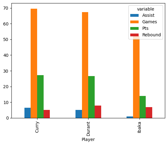
This particular visualization would be helpful if we wanted to see which stats for which each player is strongest.

For example, we can see that Steph Curry scores far more points than he does rebound, but Serge Ibaka is a bit more balanced.

What if we wanted to be able to compare all players for each statistic?

This would be easier to do if the bars were grouped by variable, with a different bar for each player.

To plot this, we need to have the variables on the index and the player name as column names.

We can get this DataFrame by setting level="Player" when calling unstack.

player_stats.unstack(level="Player")

Player	Curry	Durant	Ibaka
variable
Assist	6.466667	5.066667	0.866667
Games	69.666667	67.333333	52.333333
Pts	27.266667	26.566667	13.966667
Rebound	5.000000	7.766667	6.800000

player_stats.unstack(level="Player").plot.bar()

<Axes: xlabel='variable'>

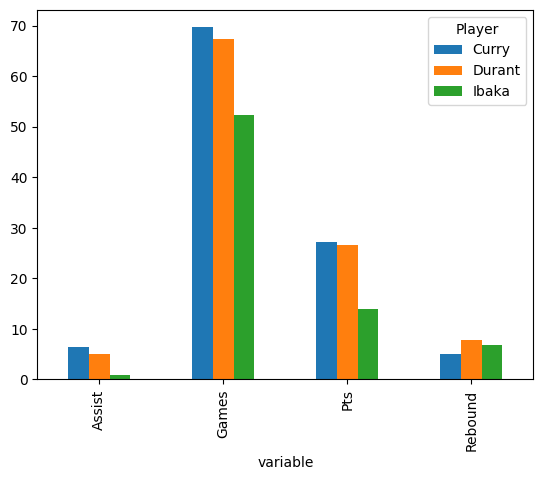
Now we can use the chart to make a number of statements about players:

• Ibaka does not get many assists, compared to Curry and Durant.

• Steph and Kevin Durant are both high scorers.

Based on the examples above, notice a few things about unstack:

• It is the inverse of stack; stack will move labels down from columns to index, while unstack moves them up from index to columns.

• By default, unstack will move the level of the index closest to the data and place it in the column labels closest to the data.

Note

Just as we can pass multiple levels to stack, we can also pass multiple levels to unstack.

We needed to use this in our solution to the exercise below.

Exercise

See exercise 1 in the exercise list.

Summary

In some ways set_index, reset_index, stack, and unstack are the “most fundamental” reshaping operations…

The other operations we discuss can be formulated with these four operations (and, in fact, some of them are exactly written as these operations in pandas’s code base).

Pro tip: We remember stack vs unstack with a mnemonic: Unstack moves index levels Up

melt

The melt method is used to move from wide to long form.

It can be used to move all of the “values” stored in your DataFrame to a single column with all other columns being used to contain identifying information.

Warning

When you use melt, any index that you currently have will be deleted.

We saw used melt above when we constructed bball_long:

bball

	Year	Player	Team	TeamName	Games	Pts	Assist	Rebound
0	2015	Curry	GSW	Warriors	79	30.1	6.7	5.4
1	2016	Curry	GSW	Warriors	79	25.3	6.6	4.5
2	2017	Curry	GSW	Warriors	51	26.4	6.1	5.1
3	2015	Durant	OKC	Thunder	72	28.2	5.0	8.2
4	2016	Durant	GSW	Warriors	62	25.1	4.8	8.3
5	2017	Durant	GSW	Warriors	68	26.4	5.4	6.8
6	2015	Ibaka	OKC	Thunder	78	12.6	0.8	6.8
7	2016	Ibaka	ORL	Magic	56	15.1	1.1	6.8
8	2016	Ibaka	TOR	Raptors	23	14.2	0.7	6.8

# this is how we made ``bball_long``
bball.melt(id_vars=["Year", "Player", "Team", "TeamName"])

	Year	Player	Team	TeamName	variable	value
0	2015	Curry	GSW	Warriors	Games	79.0
1	2016	Curry	GSW	Warriors	Games	79.0
2	2017	Curry	GSW	Warriors	Games	51.0
3	2015	Durant	OKC	Thunder	Games	72.0
4	2016	Durant	GSW	Warriors	Games	62.0
5	2017	Durant	GSW	Warriors	Games	68.0
6	2015	Ibaka	OKC	Thunder	Games	78.0
7	2016	Ibaka	ORL	Magic	Games	56.0
8	2016	Ibaka	TOR	Raptors	Games	23.0
9	2015	Curry	GSW	Warriors	Pts	30.1
10	2016	Curry	GSW	Warriors	Pts	25.3
11	2017	Curry	GSW	Warriors	Pts	26.4
12	2015	Durant	OKC	Thunder	Pts	28.2
13	2016	Durant	GSW	Warriors	Pts	25.1
14	2017	Durant	GSW	Warriors	Pts	26.4
15	2015	Ibaka	OKC	Thunder	Pts	12.6
16	2016	Ibaka	ORL	Magic	Pts	15.1
17	2016	Ibaka	TOR	Raptors	Pts	14.2
18	2015	Curry	GSW	Warriors	Assist	6.7
19	2016	Curry	GSW	Warriors	Assist	6.6
20	2017	Curry	GSW	Warriors	Assist	6.1
21	2015	Durant	OKC	Thunder	Assist	5.0
22	2016	Durant	GSW	Warriors	Assist	4.8
23	2017	Durant	GSW	Warriors	Assist	5.4
24	2015	Ibaka	OKC	Thunder	Assist	0.8
25	2016	Ibaka	ORL	Magic	Assist	1.1
26	2016	Ibaka	TOR	Raptors	Assist	0.7
27	2015	Curry	GSW	Warriors	Rebound	5.4
28	2016	Curry	GSW	Warriors	Rebound	4.5
29	2017	Curry	GSW	Warriors	Rebound	5.1
30	2015	Durant	OKC	Thunder	Rebound	8.2
31	2016	Durant	GSW	Warriors	Rebound	8.3
32	2017	Durant	GSW	Warriors	Rebound	6.8
33	2015	Ibaka	OKC	Thunder	Rebound	6.8
34	2016	Ibaka	ORL	Magic	Rebound	6.8
35	2016	Ibaka	TOR	Raptors	Rebound	6.8

Notice that the columns we specified as id_vars remained columns, but all other columns were put into two new columns:

1. variable: This has dtype string and contains the former column names. as values

2. value: This has the former values.

Using this method is an effective way to get our data in tidy form as noted above.

Exercise

See exercise 2 in the exercise list.

pivot and pivot_table

The next two reshaping methods that we will use are closely related.

Some of you might even already be familiar with these ideas because you have previously used pivot tables in Excel.

• If so, good news. We think this is even more powerful than Excel and easier to use!

• If not, good news. You are about to learn a very powerful and user-friendly tool.

We will begin with pivot.

The pivot method:

• Takes the unique values of one column and places them along the index.

• Takes the unique values of another column and places them along the columns.

• Takes the values that correspond to a third column and fills in the DataFrame values that correspond to that index/column pair.

We’ll illustrate with an example.

# .head 6 excludes Ibaka -- will discuss why later
bball.head(6).pivot(index="Year", columns="Player", values="Pts")

Player	Curry	Durant
Year
2015	30.1	28.2
2016	25.3	25.1
2017	26.4	26.4

We can replicate pivot using three of the fundamental operations from above:

1. Call set_index with the index and columns arguments

2. Extract the values column

3. unstack the columns level of the new index

#  1---------------------------------------  2---  3----------------------
bball.head(6).set_index(["Year", "Player"])["Pts"].unstack(level="Player")

Player	Curry	Durant
Year
2015	30.1	28.2
2016	25.3	25.1
2017	26.4	26.4

One important thing to be aware of is that in order for pivot to work, the index/column pairs must be unique!

Below, we demonstrate the error that occurs when they are not unique.

# Ibaka shows up twice in 2016 because he was traded mid-season from
# the Orlando Magic to the Toronto Raptors
bball.pivot(index="Year", columns="Player", values="Pts")

---------------------------------------------------------------------------
ValueError                                Traceback (most recent call last)
Cell In[22], line 3
      1 # Ibaka shows up twice in 2016 because he was traded mid-season from
      2 # the Orlando Magic to the Toronto Raptors
----> 3 bball.pivot(index="Year", columns="Player", values="Pts")

File ~/miniconda3/envs/lecture-datascience/lib/python3.12/site-packages/pandas/core/frame.py:9339, in DataFrame.pivot(self, columns, index, values)
   9332 @Substitution("")
   9333 @Appender(_shared_docs["pivot"])
   9334 def pivot(
   9335     self, *, columns, index=lib.no_default, values=lib.no_default
   9336 ) -> DataFrame:
   9337     from pandas.core.reshape.pivot import pivot
-> 9339     return pivot(self, index=index, columns=columns, values=values)

File ~/miniconda3/envs/lecture-datascience/lib/python3.12/site-packages/pandas/core/reshape/pivot.py:570, in pivot(data, columns, index, values)
    566         indexed = data._constructor_sliced(data[values]._values, index=multiindex)
    567 # error: Argument 1 to "unstack" of "DataFrame" has incompatible type "Union
    568 # [List[Any], ExtensionArray, ndarray[Any, Any], Index, Series]"; expected
    569 # "Hashable"
--> 570 result = indexed.unstack(columns_listlike)  # type: ignore[arg-type]
    571 result.index.names = [
    572     name if name is not lib.no_default else None for name in result.index.names
    573 ]
    575 return result

File ~/miniconda3/envs/lecture-datascience/lib/python3.12/site-packages/pandas/core/series.py:4615, in Series.unstack(self, level, fill_value, sort)
   4570 """
   4571 Unstack, also known as pivot, Series with MultiIndex to produce DataFrame.
   4572 
   (...)
   4611 b    2    4
   4612 """
   4613 from pandas.core.reshape.reshape import unstack
-> 4615 return unstack(self, level, fill_value, sort)

File ~/miniconda3/envs/lecture-datascience/lib/python3.12/site-packages/pandas/core/reshape/reshape.py:517, in unstack(obj, level, fill_value, sort)
    515 if is_1d_only_ea_dtype(obj.dtype):
    516     return _unstack_extension_series(obj, level, fill_value, sort=sort)
--> 517 unstacker = _Unstacker(
    518     obj.index, level=level, constructor=obj._constructor_expanddim, sort=sort
    519 )
    520 return unstacker.get_result(
    521     obj._values, value_columns=None, fill_value=fill_value
    522 )

File ~/miniconda3/envs/lecture-datascience/lib/python3.12/site-packages/pandas/core/reshape/reshape.py:154, in _Unstacker.__init__(self, index, level, constructor, sort)
    146 if num_cells > np.iinfo(np.int32).max:
    147     warnings.warn(
    148         f"The following operation may generate {num_cells} cells "
    149         f"in the resulting pandas object.",
    150         PerformanceWarning,
    151         stacklevel=find_stack_level(),
    152     )
--> 154 self._make_selectors()

File ~/miniconda3/envs/lecture-datascience/lib/python3.12/site-packages/pandas/core/reshape/reshape.py:210, in _Unstacker._make_selectors(self)
    207 mask.put(selector, True)
    209 if mask.sum() < len(self.index):
--> 210     raise ValueError("Index contains duplicate entries, cannot reshape")
    212 self.group_index = comp_index
    213 self.mask = mask

ValueError: Index contains duplicate entries, cannot reshape

pivot_table

The pivot_table method is a generalization of pivot.

It overcomes two limitations of pivot:

1. It allows you to choose multiple columns for the index/columns/values arguments.

2. It allows you to deal with duplicate entries by having you choose how to combine them.

bball

	Year	Player	Team	TeamName	Games	Pts	Assist	Rebound
0	2015	Curry	GSW	Warriors	79	30.1	6.7	5.4
1	2016	Curry	GSW	Warriors	79	25.3	6.6	4.5
2	2017	Curry	GSW	Warriors	51	26.4	6.1	5.1
3	2015	Durant	OKC	Thunder	72	28.2	5.0	8.2
4	2016	Durant	GSW	Warriors	62	25.1	4.8	8.3
5	2017	Durant	GSW	Warriors	68	26.4	5.4	6.8
6	2015	Ibaka	OKC	Thunder	78	12.6	0.8	6.8
7	2016	Ibaka	ORL	Magic	56	15.1	1.1	6.8
8	2016	Ibaka	TOR	Raptors	23	14.2	0.7	6.8

Notice that we can replicate the functionality of pivot using pivot_table if we pass the same arguments.

bball.head(6).pivot_table(index="Year", columns="Player", values="Pts")

Player	Curry	Durant
Year
2015	30.1	28.2
2016	25.3	25.1
2017	26.4	26.4

But we can also choose multiple columns to be used in index/columns/values.

bball.pivot_table(index=["Year", "Team"], columns="Player", values="Pts")

	Player	Curry	Durant	Ibaka
Year	Team
2015	GSW	30.1	NaN	NaN
	OKC	NaN	28.2	12.6
2016	GSW	25.3	25.1	NaN
	ORL	NaN	NaN	15.1
	TOR	NaN	NaN	14.2
2017	GSW	26.4	26.4	NaN

bball.pivot_table(index="Year", columns=["Player", "Team"], values="Pts")

Player	Curry	Durant		Ibaka
Team	GSW	GSW	OKC	OKC	ORL	TOR
Year
2015	30.1	NaN	28.2	12.6	NaN	NaN
2016	25.3	25.1	NaN	NaN	15.1	14.2
2017	26.4	26.4	NaN	NaN	NaN	NaN

AND we can deal with duplicated index/column pairs.

# This produced an error
# bball.pivot(index="Year", columns="Player", values="Pts")

# This doesn't!
bball_pivoted = bball.pivot_table(index="Year", columns="Player", values="Pts")
bball_pivoted

Player	Curry	Durant	Ibaka
Year
2015	30.1	28.2	12.60
2016	25.3	25.1	14.65
2017	26.4	26.4	NaN

pivot_table handles duplicate index/column pairs using an aggregation.

By default, the aggregation is the mean.

For example, our duplicated index/column pair is ("x", 1) and had associated values of 2 and 5.

Notice that bball_pivoted.loc[2016, "Ibaka"] is (15.1 + 14.2)/2 = 14.65.

We can choose how pandas aggregates all of the values.

For example, here’s how we would keep the max.

bball.pivot_table(index="Year", columns="Player", values="Pts", aggfunc=max)

/tmp/ipykernel_2912/108613235.py:1: FutureWarning: The provided callable <built-in function max> is currently using DataFrameGroupBy.max. In a future version of pandas, the provided callable will be used directly. To keep current behavior pass the string "max" instead.
  bball.pivot_table(index="Year", columns="Player", values="Pts", aggfunc=max)

Player	Curry	Durant	Ibaka
Year
2015	30.1	28.2	12.6
2016	25.3	25.1	15.1
2017	26.4	26.4	NaN

Maybe we wanted to count how many values there were.

bball.pivot_table(index="Year", columns="Player", values="Pts", aggfunc=len)

Player	Curry	Durant	Ibaka
Year
2015	1.0	1.0	1.0
2016	1.0	1.0	2.0
2017	1.0	1.0	NaN

We can even pass multiple aggregation functions!

bball.pivot_table(index="Year", columns="Player", values="Pts", aggfunc=[max, len])

/tmp/ipykernel_2912/2429470343.py:1: FutureWarning: The provided callable <built-in function max> is currently using DataFrameGroupBy.max. In a future version of pandas, the provided callable will be used directly. To keep current behavior pass the string "max" instead.
  bball.pivot_table(index="Year", columns="Player", values="Pts", aggfunc=[max, len])

	max			len
Player	Curry	Durant	Ibaka	Curry	Durant	Ibaka
Year
2015	30.1	28.2	12.6	1.0	1.0	1.0
2016	25.3	25.1	15.1	1.0	1.0	2.0
2017	26.4	26.4	NaN	1.0	1.0	NaN

Exercise

See exercise 3 in the exercise list.

Visualizing Reshaping

Now that you have learned the basics and had a chance to experiment, we will use some generic data to provide a visualization of what the above reshape operations do.

The data we will use is:

# made up
# columns A and B are "identifiers" while C, D, and E are variables.
df = pd.DataFrame({
    "A": [0, 0, 1, 1],
    "B": "x y x z".split(),
    "C": [1, 2, 1, 4],
    "D": [10, 20, 30, 20,],
    "E": [2, 1, 5, 4,]
})

df.info()
df

<class 'pandas.core.frame.DataFrame'>
RangeIndex: 4 entries, 0 to 3
Data columns (total 5 columns):
 #   Column  Non-Null Count  Dtype 
---  ------  --------------  ----- 
 0   A       4 non-null      int64 
 1   B       4 non-null      object
 2   C       4 non-null      int64 
 3   D       4 non-null      int64 
 4   E       4 non-null      int64 
dtypes: int64(4), object(1)
memory usage: 292.0+ bytes

	A	B	C	D	E
0	0	x	1	10	2
1	0	y	2	20	1
2	1	x	1	30	5
3	1	z	4	20	4

df2 = df.set_index(["A", "B"])
df2.head()

		C	D	E
A	B
0	x	1	10	2
	y	2	20	1
1	x	1	30	5
	z	4	20	4

df3 = df2.T
df3.head()

A	0		1
B	x	y	x	z
C	1	2	1	4
D	10	20	30	20
E	2	1	5	4

stack and unstack

Below is an animation that shows how stacking works.

df2

		C	D	E
A	B
0	x	1	10	2
	y	2	20	1
1	x	1	30	5
	z	4	20	4

df2_stack = df2.stack()
df2_stack

A  B   
0  x  C     1
      D    10
      E     2
   y  C     2
      D    20
      E     1
1  x  C     1
      D    30
      E     5
   z  C     4
      D    20
      E     4
dtype: int64

And here is an animation that shows how unstacking works.

df2

		C	D	E
A	B
0	x	1	10	2
	y	2	20	1
1	x	1	30	5
	z	4	20	4

df2.unstack()

	C			D			E
B	x	y	z	x	y	z	x	y	z
A
0	1.0	2.0	NaN	10.0	20.0	NaN	2.0	1.0	NaN
1	1.0	NaN	4.0	30.0	NaN	20.0	5.0	NaN	4.0

melt

As noted above, the melt method transforms data from wide to long in form.

Here’s a visualization of that operation.

df

	A	B	C	D	E
0	0	x	1	10	2
1	0	y	2	20	1
2	1	x	1	30	5
3	1	z	4	20	4

df_melted = df.melt(id_vars=["A", "B"])
df_melted

	A	B	variable	value
0	0	x	C	1
1	0	y	C	2
2	1	x	C	1
3	1	z	C	4
4	0	x	D	10
5	0	y	D	20
6	1	x	D	30
7	1	z	D	20
8	0	x	E	2
9	0	y	E	1
10	1	x	E	5
11	1	z	E	4

Exercises

Exercise 1

Warning

This one is challenging

Recall the bball_wide DataFrame from above (repeated below to jog your memory).

In this task, you will start from ball and re-recreate bball_wide by combining the operations we just learned about.

There are many ways to do this, so be creative.

Our solution used set_index, T, stack, and unstack in that order.

Here are a few hints:

• Hint

  Think about what columns you will need to call set_index on so that their data ends up as labels (either in index or columns).

• Hint

  Leave other columns (e.g. the actual game stats) as actual columns so their data can stay data during your reshaping.

Don’t spend too much time on this… if you get stuck, you will find our answer here.

Hint

You might need to add .sort_index(axis=1) after you are finished to get the columns in the same order.

Hint

You may not end up with a variable header on the second level of column labels. This is ok.

bball_wide

(back to text)

Exercise 2

• What do you think would happen if we wrote bball.melt(id_vars=["Year", "Player"]) rather than bball.melt(id_vars=["Year", "Player", "Team", "TeamName"])? Were you right? Write your thoughts.

• Read the documentation and focus on the argument value_vars. How does bball.melt(id_vars=["Year", "Player"], value_vars=["Pts", "Rebound"]) differ from bball.melt(id_vars=["Year", "Player"])?

• Consider the differences between bball.stack and bball.melt. Is there a way to make them generate the same output? Write your thoughts.

  • Hint

    You might need to use both stack and another method from above

(back to text)

Exercise 3

• First, take a breath… That was a lot to take in.

• Can you think of a reason to ever use pivot rather than pivot_table? Write your thoughts.

• Create a pivot table with column Player as the index, TeamName as the columns, and [Rebound, Assist] as the values. What happens when you use aggfunc=[np.max, np.min, len]? Describe how Python produced each of the values in the resultant pivot table.

(back to text)