Merge#

Prerequisites

Reshape

Outcomes

Know the different pandas routines for combining datasets
Know when to use pd.concat vs pd.merge vs pd.join
Be able to apply the three main combining routines

Data

WDI data on GDP components, population, and square miles of countries
Book ratings: 6,000,000 ratings for the 10,000 most rated books on Goodreads
Details for all delayed US domestic flights in November 2016, obtained from the Bureau of Transportation Statistics

# Uncomment following line to install on colab
#! pip install 

Combining Datasets#

Often, we will want perform joint analysis on data from different sources.

For example, when analyzing the regional sales for a company, we might want to include industry aggregates or demographic information for each region.

Or perhaps we are working with product-level data, have a list of product groups in a separate dataset, and want to compute aggregate statistics for each group.

import pandas as pd
%matplotlib inline

from IPython.display import display

# from WDI. Units trillions of 2010 USD
url = "https://datascience.quantecon.org/assets/data/wdi_data.csv"
wdi = pd.read_csv(url).set_index(["country", "year"])
wdi.info()

wdi2017 = wdi.xs(2017, level="year")
wdi2017

<class 'pandas.core.frame.DataFrame'>
MultiIndex: 72 entries, ('Canada', 2017) to ('United States', 2000)
Data columns (total 5 columns):
 #   Column       Non-Null Count  Dtype  
---  ------       --------------  -----  
 0   GovExpend    72 non-null     float64
 1   Consumption  72 non-null     float64
 2   Exports      72 non-null     float64
 3   Imports      72 non-null     float64
 4   GDP          72 non-null     float64
dtypes: float64(5)
memory usage: 3.9+ KB

	GovExpend	Consumption	Exports	Imports	GDP
country
Canada	0.372665	1.095475	0.582831	0.600031	1.868164
Germany	0.745579	2.112009	1.930563	1.666348	3.883870
United Kingdom	0.549538	1.809154	0.862629	0.933145	2.818704
United States	2.405743	12.019266	2.287071	3.069954	17.348627

wdi2016_17 = wdi.loc[pd.IndexSlice[:, [2016, 2017]],: ]
wdi2016_17

		GovExpend	Consumption	Exports	Imports	GDP
country	year
Canada	2016	0.364899	1.058426	0.576394	0.575775	1.814016
Germany	2016	0.734014	2.075615	1.844949	1.589495	3.801859
United Kingdom	2016	0.550596	1.772348	0.816792	0.901494	2.768241
United States	2016	2.407981	11.722133	2.219937	2.936004	16.972348
Canada	2017	0.372665	1.095475	0.582831	0.600031	1.868164
Germany	2017	0.745579	2.112009	1.930563	1.666348	3.883870
United Kingdom	2017	0.549538	1.809154	0.862629	0.933145	2.818704
United States	2017	2.405743	12.019266	2.287071	3.069954	17.348627

# Data from https://www.nationmaster.com/country-info/stats/Geography/Land-area/Square-miles
# units -- millions of square miles
sq_miles = pd.Series({
   "United States": 3.8,
   "Canada": 3.8,
   "Germany": 0.137,
   "United Kingdom": 0.0936,
   "Russia": 6.6,
}, name="sq_miles").to_frame()
sq_miles.index.name = "country"
sq_miles

	sq_miles
country
United States	3.8000
Canada	3.8000
Germany	0.1370
United Kingdom	0.0936
Russia	6.6000

# from WDI. Units millions of people
pop_url = "https://datascience.quantecon.org/assets/data/wdi_population.csv"
pop = pd.read_csv(pop_url).set_index(["country", "year"])
pop.info()
pop.head(10)

<class 'pandas.core.frame.DataFrame'>
MultiIndex: 72 entries, ('Canada', 2017) to ('United States', 2000)
Data columns (total 1 columns):
 #   Column      Non-Null Count  Dtype  
---  ------      --------------  -----  
 0   Population  72 non-null     float64
dtypes: float64(1)
memory usage: 1.7+ KB

		Population
country	year
Canada	2017	36.540268
	2016	36.109487
	2015	35.702908
	2014	35.437435
	2013	35.082954
	2012	34.714222
	2011	34.339328
	2010	34.004889
	2009	33.628895
	2008	33.247118

Suppose that we were asked to compute a number of statistics with the data above:

As a measure of land usage or productivity, what is Consumption per square mile?
What is GDP per capita (per person) for each country in each year? How about Consumption per person?
What is the population density of each country? How much does it change over time?

Notice that to answer any of the questions from above, we will have to use data from more than one of our DataFrames.

In this lecture, we will learn many techniques for combining datasets that originate from different sources, careful to ensure that data is properly aligned.

In pandas three main methods can combine datasets:

pd.concat([dfs...])
pd.merge(df1, df2)
df1.join(df2)

We’ll look at each one.

`pd.concat`#

The pd.concat function is used to stack two or more DataFrames together.

An example of when you might want to do this is if you have monthly data in separate files on your computer and would like to have 1 year of data in a single DataFrame.

The first argument to pd.concat is a list of DataFrames to be stitched together.

The other commonly used argument is named axis.

As we have seen before, many pandas functions have an axis argument that specifies whether a particular operation should happen down rows (axis=0) or along columns (axis=1).

In the context of pd.concat, setting axis=0 (the default case) will stack DataFrames on top of one another while axis=1 stacks them side by side.

We’ll look at each case separately.

`axis=0`#

When we call pd.concat and set axis=0, the list of DataFrames passed in the first argument will be stacked on top of one another.

Let’s try it out here.

# equivalent to pd.concat([wdi2017, sq_miles]) -- axis=0 is default
pd.concat([wdi2017, sq_miles], axis=0)

	GovExpend	Consumption	Exports	Imports	GDP	sq_miles
country
Canada	0.372665	1.095475	0.582831	0.600031	1.868164	NaN
Germany	0.745579	2.112009	1.930563	1.666348	3.883870	NaN
United Kingdom	0.549538	1.809154	0.862629	0.933145	2.818704	NaN
United States	2.405743	12.019266	2.287071	3.069954	17.348627	NaN
United States	NaN	NaN	NaN	NaN	NaN	3.8000
Canada	NaN	NaN	NaN	NaN	NaN	3.8000
Germany	NaN	NaN	NaN	NaN	NaN	0.1370
United Kingdom	NaN	NaN	NaN	NaN	NaN	0.0936
Russia	NaN	NaN	NaN	NaN	NaN	6.6000

Notice a few things:

The number of rows in the output is the total number : of rows in all inputs. The labels are all from the original DataFrames.

The column labels are all the distinct column labels from all the inputs.
For columns that appeared only in one input, the value for all row labels originating from a different input is equal to NaN (marked as missing).

`axis=1`#

In this example, concatenating by stacking side-by-side makes more sense.

We accomplish this by passing axis=1 to pd.concat:

pd.concat([wdi2017, sq_miles], axis=1)

	GovExpend	Consumption	Exports	Imports	GDP	sq_miles
country
Canada	0.372665	1.095475	0.582831	0.600031	1.868164	3.8000
Germany	0.745579	2.112009	1.930563	1.666348	3.883870	0.1370
United Kingdom	0.549538	1.809154	0.862629	0.933145	2.818704	0.0936
United States	2.405743	12.019266	2.287071	3.069954	17.348627	3.8000
Russia	NaN	NaN	NaN	NaN	NaN	6.6000

Notice here that

The index entries are all unique index entries that appeared in any DataFrame.
The column labels are all column labels from the inputs.
As wdi2017 didn’t have a Russia row, the value for all of its columns is NaN.

Now we can answer one of our questions from above: What is Consumption per square mile?

temp = pd.concat([wdi2017, sq_miles], axis=1)
temp["Consumption"] / temp["sq_miles"]

country
Canada             0.288283
Germany           15.416124
United Kingdom    19.328569
United States      3.162965
Russia                  NaN
dtype: float64

Since the WDI data is measured in millions of US Dollars, this gives us the consumption per square mile measured in units of millions of USD per square mile.

`pd.merge`#

pd.merge operates on two DataFrames at a time and is primarily used to bring columns from one DataFrame into another, aligning data based on one or more “key” columns.

This is a somewhat difficult concept to grasp by reading, so let’s look at some examples.

pd.merge(wdi2017, sq_miles, on="country")

	GovExpend	Consumption	Exports	Imports	GDP	sq_miles
country
Canada	0.372665	1.095475	0.582831	0.600031	1.868164	3.8000
Germany	0.745579	2.112009	1.930563	1.666348	3.883870	0.1370
United Kingdom	0.549538	1.809154	0.862629	0.933145	2.818704	0.0936
United States	2.405743	12.019266	2.287071	3.069954	17.348627	3.8000

The output here looks very similar to what we saw with concat and axis=1, except that the row for Russia does not appear.

We will talk more about why this happened soon.

For now, let’s look at a slightly more intriguing example:

pd.merge(wdi2016_17, sq_miles, on="country")

	GovExpend	Consumption	Exports	Imports	GDP	sq_miles
country
Canada	0.364899	1.058426	0.576394	0.575775	1.814016	3.8000
Germany	0.734014	2.075615	1.844949	1.589495	3.801859	0.1370
United Kingdom	0.550596	1.772348	0.816792	0.901494	2.768241	0.0936
United States	2.407981	11.722133	2.219937	2.936004	16.972348	3.8000
Canada	0.372665	1.095475	0.582831	0.600031	1.868164	3.8000
Germany	0.745579	2.112009	1.930563	1.666348	3.883870	0.1370
United Kingdom	0.549538	1.809154	0.862629	0.933145	2.818704	0.0936
United States	2.405743	12.019266	2.287071	3.069954	17.348627	3.8000

Here’s how we think about what happened:

The data in wdi2016_17 is copied over exactly as is.
Because country was on the index for both DataFrames, it is on the index of the output.
We lost the year on the index – we’ll work on getting it back below.
The additional column in sq_miles was added to column labels for the output.
The data from the sq_miles column was added to the output by looking up rows where the country in the two DataFrames lined up.
- Note that all the countries appeared twice, and the data in sq_miles was repeated. This is because wdi2016_17 had two rows for each country.
- Also note that because Russia did not appear in wdi2016_17, the value sq_miles.loc["Russia"] (i.e. 6.6) is not used the output.

How do we get the year back?

We must first call reset_index on wdi2016_17 so that in the first step when all columns are copied over, year is included.

pd.merge(wdi2016_17.reset_index(), sq_miles, on="country")

	country	year	GovExpend	Consumption	Exports	Imports	GDP	sq_miles
0	Canada	2016	0.364899	1.058426	0.576394	0.575775	1.814016	3.8000
1	Germany	2016	0.734014	2.075615	1.844949	1.589495	3.801859	0.1370
2	United Kingdom	2016	0.550596	1.772348	0.816792	0.901494	2.768241	0.0936
3	United States	2016	2.407981	11.722133	2.219937	2.936004	16.972348	3.8000
4	Canada	2017	0.372665	1.095475	0.582831	0.600031	1.868164	3.8000
5	Germany	2017	0.745579	2.112009	1.930563	1.666348	3.883870	0.1370
6	United Kingdom	2017	0.549538	1.809154	0.862629	0.933145	2.818704	0.0936
7	United States	2017	2.405743	12.019266	2.287071	3.069954	17.348627	3.8000

Multiple Columns#

Sometimes, we need to merge multiple columns.

For example our pop and wdi2016_17 DataFrames both have observations organized by country and year.

To properly merge these datasets, we would need to align the data by both country and year.

We pass a list to the on argument to accomplish this:

pd.merge(wdi2016_17, pop, on=["country", "year"])

		GovExpend	Consumption	Exports	Imports	GDP	Population
country	year
Canada	2016	0.364899	1.058426	0.576394	0.575775	1.814016	36.109487
Germany	2016	0.734014	2.075615	1.844949	1.589495	3.801859	82.348669
United Kingdom	2016	0.550596	1.772348	0.816792	0.901494	2.768241	65.595565
United States	2016	2.407981	11.722133	2.219937	2.936004	16.972348	323.071342
Canada	2017	0.372665	1.095475	0.582831	0.600031	1.868164	36.540268
Germany	2017	0.745579	2.112009	1.930563	1.666348	3.883870	82.657002
United Kingdom	2017	0.549538	1.809154	0.862629	0.933145	2.818704	66.058859
United States	2017	2.405743	12.019266	2.287071	3.069954	17.348627	325.147121

Now, we can answer more of our questions from above: What is GDP per capita (per person) for each country in each year? How about Consumption per person?

wdi_pop = pd.merge(wdi2016_17, pop, on=["country", "year"])
wdi_pop["GDP"] / wdi_pop["Population"]

country         year
Canada          2016    0.050237
Germany         2016    0.046168
United Kingdom  2016    0.042202
United States   2016    0.052534
Canada          2017    0.051126
Germany         2017    0.046988
United Kingdom  2017    0.042670
United States   2017    0.053356
dtype: float64

wdi_pop["Consumption"] / wdi_pop["Population"]

country         year
Canada          2016    0.029312
Germany         2016    0.025205
United Kingdom  2016    0.027019
United States   2016    0.036283
Canada          2017    0.029980
Germany         2017    0.025551
United Kingdom  2017    0.027387
United States   2017    0.036966
dtype: float64

These numbers tell us the GDP and consumption per capita, measured in units of millions of USD per person.

Exercise

See exercise 1 in the exercise list.

Arguments to `merge`#

The pd.merge function can take many optional arguments.

We’ll talk about a few of the most commonly-used ones here and refer you to the documentation for more details.

We’ll follow the pandas convention and refer to the first argument to pd.merge as left and call the second right.

`on`#

We have already seen this one used before, but we want to point out that on is optional.

If nothing is given for this argument, pandas will use all columns in left and right with the same name.

In our example, country is the only column that appears in both DataFrames, so it is used for on if we don’t pass anything.

The following two are equivalent.

pd.merge(wdi2017, sq_miles, on="country")

	GovExpend	Consumption	Exports	Imports	GDP	sq_miles
country
Canada	0.372665	1.095475	0.582831	0.600031	1.868164	3.8000
Germany	0.745579	2.112009	1.930563	1.666348	3.883870	0.1370
United Kingdom	0.549538	1.809154	0.862629	0.933145	2.818704	0.0936
United States	2.405743	12.019266	2.287071	3.069954	17.348627	3.8000

# if we move index back to columns, the `on` is un-necessary
pd.merge(wdi2017.reset_index(), sq_miles.reset_index())

	country	GovExpend	Consumption	Exports	Imports	GDP	sq_miles
0	Canada	0.372665	1.095475	0.582831	0.600031	1.868164	3.8000
1	Germany	0.745579	2.112009	1.930563	1.666348	3.883870	0.1370
2	United Kingdom	0.549538	1.809154	0.862629	0.933145	2.818704	0.0936
3	United States	2.405743	12.019266	2.287071	3.069954	17.348627	3.8000

`left_on`, `right_on`#

Above, we used the on argument to identify a column in both left and right that was used to align data.

Sometimes, both DataFrames don’t have the same name for this column.

In that case, we use the left_on and right_on arguments, passing the proper column name(s) to align the data.

We’ll show you an example below, but it is somewhat silly as our DataFrames do both have the country column.

pd.merge(wdi2017, sq_miles, left_on="country", right_on="country")

	GovExpend	Consumption	Exports	Imports	GDP	sq_miles
country
Canada	0.372665	1.095475	0.582831	0.600031	1.868164	3.8000
Germany	0.745579	2.112009	1.930563	1.666348	3.883870	0.1370
United Kingdom	0.549538	1.809154	0.862629	0.933145	2.818704	0.0936
United States	2.405743	12.019266	2.287071	3.069954	17.348627	3.8000

`left_index`, `right_index`#

Sometimes, as in our example, the key used to align data is actually in the index instead of one of the columns.

In this case, we can use the left_index or right_index arguments.

We should only set these values to a boolean (True or False).

Let’s practice with this.

pd.merge(wdi2017, sq_miles, left_on="country", right_index=True)

	GovExpend	Consumption	Exports	Imports	GDP	sq_miles
country
Canada	0.372665	1.095475	0.582831	0.600031	1.868164	3.8000
Germany	0.745579	2.112009	1.930563	1.666348	3.883870	0.1370
United Kingdom	0.549538	1.809154	0.862629	0.933145	2.818704	0.0936
United States	2.405743	12.019266	2.287071	3.069954	17.348627	3.8000

`how`#

The how is perhaps the most powerful, but most conceptually difficult of the arguments we will cover.

This argument controls which values from the key column(s) appear in the output.

The 4 possible options for this argument are summarized in the image below.

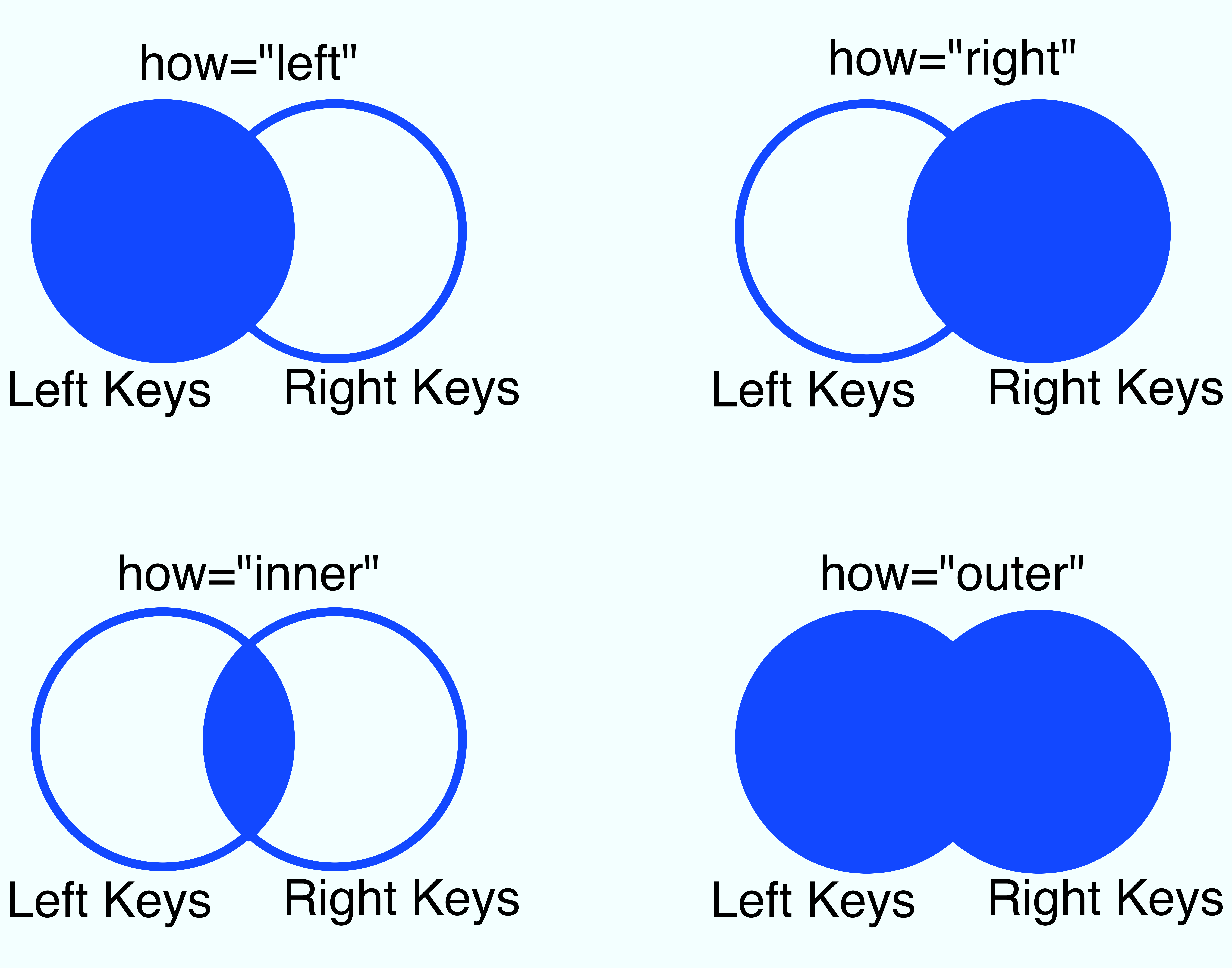
In words, we have:

left: What we described above. It uses the keys from the left DataFrame.
right: Output will contain all keys from right.
inner: The default how; the output will only contain keys that appear in both left and right.
outer: The output will contain any key found in either left or right.

In addition to the above, we will use the following two DataFrames to illustrate the how option.

wdi2017_no_US = wdi2017.drop("United States")
wdi2017_no_US

	GovExpend	Consumption	Exports	Imports	GDP
country
Canada	0.372665	1.095475	0.582831	0.600031	1.868164
Germany	0.745579	2.112009	1.930563	1.666348	3.883870
United Kingdom	0.549538	1.809154	0.862629	0.933145	2.818704

sq_miles_no_germany = sq_miles.drop("Germany")
sq_miles_no_germany

	sq_miles
country
United States	3.8000
Canada	3.8000
United Kingdom	0.0936
Russia	6.6000

Now, let’s see all the possible how options.

# default
pd.merge(wdi2017, sq_miles, on="country", how="left")

	GovExpend	Consumption	Exports	Imports	GDP	sq_miles
country
Canada	0.372665	1.095475	0.582831	0.600031	1.868164	3.8000
Germany	0.745579	2.112009	1.930563	1.666348	3.883870	0.1370
United Kingdom	0.549538	1.809154	0.862629	0.933145	2.818704	0.0936
United States	2.405743	12.019266	2.287071	3.069954	17.348627	3.8000

# notice ``Russia`` is included
pd.merge(wdi2017, sq_miles, on="country", how="right")

	GovExpend	Consumption	Exports	Imports	GDP	sq_miles
country
United States	2.405743	12.019266	2.287071	3.069954	17.348627	3.8000
Canada	0.372665	1.095475	0.582831	0.600031	1.868164	3.8000
Germany	0.745579	2.112009	1.930563	1.666348	3.883870	0.1370
United Kingdom	0.549538	1.809154	0.862629	0.933145	2.818704	0.0936
Russia	NaN	NaN	NaN	NaN	NaN	6.6000

# notice no United States or Russia
pd.merge(wdi2017_no_US, sq_miles, on="country", how="inner")

	GovExpend	Consumption	Exports	Imports	GDP	sq_miles
country
Canada	0.372665	1.095475	0.582831	0.600031	1.868164	3.8000
Germany	0.745579	2.112009	1.930563	1.666348	3.883870	0.1370
United Kingdom	0.549538	1.809154	0.862629	0.933145	2.818704	0.0936

# includes all 5, even though they don't all appear in either DataFrame
pd.merge(wdi2017_no_US, sq_miles_no_germany, on="country", how="outer")

	GovExpend	Consumption	Exports	Imports	GDP	sq_miles
country
Canada	0.372665	1.095475	0.582831	0.600031	1.868164	3.8000
Germany	0.745579	2.112009	1.930563	1.666348	3.883870	NaN
Russia	NaN	NaN	NaN	NaN	NaN	6.6000
United Kingdom	0.549538	1.809154	0.862629	0.933145	2.818704	0.0936
United States	NaN	NaN	NaN	NaN	NaN	3.8000

Exercise

See exercise 2 in the exercise list.

Exercise

See exercise 3 in the exercise list.

`df.merge(df2)`#

Note that the DataFrame type has a merge method.

It is the same as the function we have been working with, but passes the DataFrame before the period as left.

Thus df.merge(other) is equivalent to pd.merge(df, other).

wdi2017.merge(sq_miles, on="country", how="right")

	GovExpend	Consumption	Exports	Imports	GDP	sq_miles
country
United States	2.405743	12.019266	2.287071	3.069954	17.348627	3.8000
Canada	0.372665	1.095475	0.582831	0.600031	1.868164	3.8000
Germany	0.745579	2.112009	1.930563	1.666348	3.883870	0.1370
United Kingdom	0.549538	1.809154	0.862629	0.933145	2.818704	0.0936
Russia	NaN	NaN	NaN	NaN	NaN	6.6000

`df.join`#

The join method for a DataFrame is very similar to the merge method described above, but only allows you to use the index of the right DataFrame as the join key.

Thus, left.join(right, on="country") is equivalent to calling pd.merge(left, right, left_on="country", right_index=True).

The implementation of the join method calls merge internally, but sets the left_on and right_index arguments for you.

You can do anything with df.join that you can do with df.merge, but df.join is more convenient to use if the keys of right are in the index.

wdi2017.join(sq_miles, on="country")

	GovExpend	Consumption	Exports	Imports	GDP	sq_miles
country
Canada	0.372665	1.095475	0.582831	0.600031	1.868164	3.8000
Germany	0.745579	2.112009	1.930563	1.666348	3.883870	0.1370
United Kingdom	0.549538	1.809154	0.862629	0.933145	2.818704	0.0936
United States	2.405743	12.019266	2.287071	3.069954	17.348627	3.8000

wdi2017.merge(sq_miles, left_on="country", right_index=True)

	GovExpend	Consumption	Exports	Imports	GDP	sq_miles
country
Canada	0.372665	1.095475	0.582831	0.600031	1.868164	3.8000
Germany	0.745579	2.112009	1.930563	1.666348	3.883870	0.1370
United Kingdom	0.549538	1.809154	0.862629	0.933145	2.818704	0.0936
United States	2.405743	12.019266	2.287071	3.069954	17.348627	3.8000

Case Study#

Let’s put these tools to practice by loading some real datasets and seeing how these functions can be applied.

We’ll analyze ratings of books from the website Goodreads.

We accessed the data here.

Let’s load it up.

url = "https://datascience.quantecon.org/assets/data/goodreads_ratings.csv.zip"
ratings = pd.read_csv(url)
display(ratings.head())
ratings.info()

	Unnamed: 0	user_id	book_id	rating
0	0	1	258	5
1	1	2	4081	4
2	2	2	260	5
3	3	2	9296	5
4	4	2	2318	3

<class 'pandas.core.frame.DataFrame'>
RangeIndex: 5976479 entries, 0 to 5976478
Data columns (total 4 columns):
 #   Column      Dtype
---  ------      -----
 0   Unnamed: 0  int64
 1   user_id     int64
 2   book_id     int64
 3   rating      int64
dtypes: int64(4)
memory usage: 182.4 MB

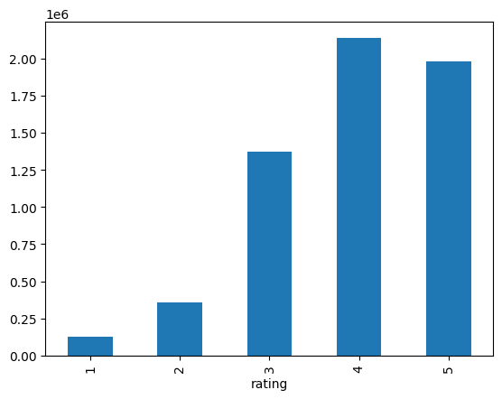
We can already do some interesting things with just the ratings data.

Let’s see how many ratings of each number are in our dataset.

ratings["rating"].value_counts().sort_index().plot(kind="bar");

../_images/707dba01643e99c9b1351fefd6f10c0a24d358831bdabf052ca5f626c9d762ce.png

Let’s also see how many users have rated N books, for all N possible.

To do this, we will use value_counts twice (can you think of why?).

We will see a more flexible way of performing similar grouped operations in a future lecture.

users_by_n = (
    ratings["user_id"]
    .value_counts()  # Series called "count". Index: user_id, value: n ratings by user
    .rename("N_ratings")  # Rename the Series to "N_ratings"
    .value_counts()  # Series called "count". Index: n_ratings by user, value: N_users with this many ratings
    .sort_index()    # Sort our Series by the index (number of ratings)
    .reset_index()   # Dataframe with columns `index` (from above) and `user_id`
    .rename(columns={"count": "N_users"})
    .set_index("N_ratings")
)
users_by_n.head(10)

	N_users
N_ratings
19	1
20	1
21	3
22	13
23	5
24	11
25	13
26	23
27	34
28	26

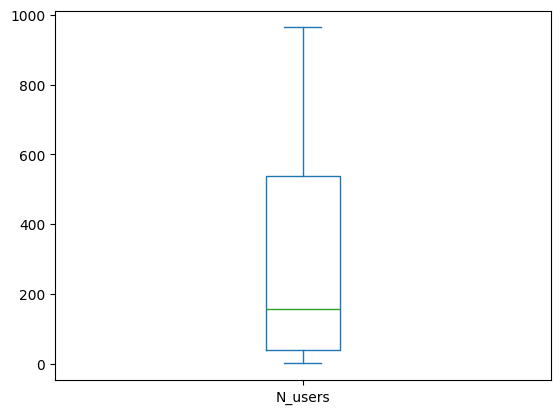
Let’s look at some statistics on that dataset.

users_by_n.describe()

	N_users
count	181.000000
mean	295.160221
std	309.461848
min	1.000000
25%	40.000000
50%	158.000000
75%	538.000000
max	964.000000

We can see the same data visually in a box plot.

users_by_n.plot(kind="box", subplots=True)

N_users    Axes(0.125,0.11;0.775x0.77)
dtype: object

../_images/14569e67694b7c2280ce41a82c21328572005343dd1e865efde407bdbc386be0.png

Let’s practice applying the want operator…

Want: Determine whether a relationship between the number of ratings a user has written and the distribution of the ratings exists. (Maybe we are an author hoping to inflate our ratings and wonder if we should target “more experienced” Goodreads users, or focus on newcomers.)

Let’s start from the result and work our way backwards:

We can answer our question if we have two similar DataFrames:
- All ratings by the N (e.g. 5) users with the most ratings
- All ratings by the N users with the least number of ratings
To get that, we will need to extract rows of ratings with user_id associated with the N most and least prolific raters
For that, we need the most and least active user_ids
To get that info, we need a count of how many ratings each user left.
- We can get that with df["user_id"].value_counts(), so let’s start there.

# step 4
n_ratings = ratings["user_id"].value_counts()
n_ratings.head()

user_id
  200
  200
  199
  199
  199
Name: count, dtype: int64

# step 3
N = 5
most_prolific_users = n_ratings.nlargest(5).index.tolist()
least_prolific_users = n_ratings.nsmallest(5).index.tolist()

# step 2
active_ratings = ratings.loc[ratings["user_id"].isin(most_prolific_users), :]
inactive_ratings = ratings.loc[ratings["user_id"].isin(least_prolific_users), :]

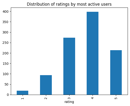
# step 1 -- get the answer!
active_ratings["rating"].value_counts().sort_index().plot(
    kind="bar", title="Distribution of ratings by most active users"
)

<Axes: title={'center': 'Distribution of ratings by most active users'}, xlabel='rating'>

../_images/208a099e3edd0ed035af70b31554317a220b77df586b4f67c55510f427494ee5.png

inactive_ratings["rating"].value_counts().sort_index().plot(
    kind="bar", title="Distribution of ratings by least active users"
)

<Axes: title={'center': 'Distribution of ratings by least active users'}, xlabel='rating'>

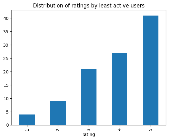
../_images/5af6d2f5522d32eebdeea5b8c611fb9b3147363a743915bd74ac44afe034381a.png

Nice! From the picture above, the new users look much more likely to leave 5 star ratings than more experienced users.

Book Data#

We know what you are probably thinking: “Isn’t this a lecture on merging? Why are we only using one dataset?”

We hear you.

Let’s also load a dataset containing information on the actual books.

url = "https://datascience.quantecon.org/assets/data/goodreads_books.csv"
books = pd.read_csv(url)
# we only need a few of the columns
books = books[["book_id", "authors", "title"]]
print("shape: ", books.shape)
print("dtypes:\n", books.dtypes, sep="")
books.head()

shape:  (10000, 3)
dtypes:
book_id     int64
authors    object
title      object
dtype: object

	book_id	authors	title
0	1	Suzanne Collins	The Hunger Games (The Hunger Games, #1)
1	2	J.K. Rowling, Mary GrandPré	Harry Potter and the Sorcerer's Stone (Harry P...
2	3	Stephenie Meyer	Twilight (Twilight, #1)
3	4	Harper Lee	To Kill a Mockingbird
4	5	F. Scott Fitzgerald	The Great Gatsby

We could do similar interesting things with just the books dataset, but we will skip it for now and merge them together.

rated_books = pd.merge(ratings, books)

Now, let’s see which books have been most often rated.

most_rated_books_id = rated_books["book_id"].value_counts().nlargest(10).index
most_rated_books = rated_books.loc[rated_books["book_id"].isin(most_rated_books_id), :]
list(most_rated_books["title"].unique())

['Harry Potter and the Prisoner of Azkaban (Harry Potter, #3)',
 "Harry Potter and the Sorcerer's Stone (Harry Potter, #1)",
 'Harry Potter and the Chamber of Secrets (Harry Potter, #2)',
 'The Great Gatsby',
 'To Kill a Mockingbird',
 'The Hobbit',
 'Twilight (Twilight, #1)',
 'The Hunger Games (The Hunger Games, #1)',
 'Catching Fire (The Hunger Games, #2)',
 'Mockingjay (The Hunger Games, #3)']

Let’s use our pivot_table knowledge to compute the average rating for each of these books.

most_rated_books.pivot_table(values="rating", index="title")

	rating
title
Catching Fire (The Hunger Games, #2)	4.133422
Harry Potter and the Chamber of Secrets (Harry Potter, #2)	4.229418
Harry Potter and the Prisoner of Azkaban (Harry Potter, #3)	4.418732
Harry Potter and the Sorcerer's Stone (Harry Potter, #1)	4.351350
Mockingjay (The Hunger Games, #3)	3.853131
The Great Gatsby	3.772224
The Hobbit	4.148477
The Hunger Games (The Hunger Games, #1)	4.279707
To Kill a Mockingbird	4.329369
Twilight (Twilight, #1)	3.214341

These ratings seem surprisingly low, given that they are the most often rated books on Goodreads.

I wonder what the bottom of the distribution looks like…

Exercise

See exercise 4 in the exercise list.

Let’s compute the average number of ratings for each book in our sample.

average_ratings = (
    rated_books
    .pivot_table(values="rating", index="title")
    .sort_values(by="rating", ascending=False)
)
average_ratings.head(10)

	rating
title
The Complete Calvin and Hobbes	4.829876
ESV Study Bible	4.818182
Attack of the Deranged Mutant Killer Monster Snow Goons	4.768707
The Indispensable Calvin and Hobbes	4.766355
The Revenge of the Baby-Sat	4.761364
There's Treasure Everywhere: A Calvin and Hobbes Collection	4.760456
The Authoritative Calvin and Hobbes: A Calvin and Hobbes Treasury	4.757202
It's a Magical World: A Calvin and Hobbes Collection	4.747396
Harry Potter Boxed Set, Books 1-5 (Harry Potter, #1-5)	4.736842
The Calvin and Hobbes Tenth Anniversary Book	4.728528

What does the overall distribution of average ratings look like?

# plot a kernel density estimate of average ratings
average_ratings.plot.density(xlim=(1, 5))

# or a histogram
average_ratings.plot.hist(bins=30, xlim=(1, 5))

<Axes: ylabel='Frequency'>

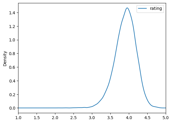
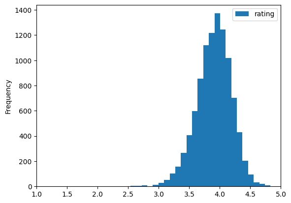
../_images/58a138482ba639dd90c6bf0aedbf40bd39a091881f5854f56865dfd8a064717f.png

../_images/053395fe1b39253cf710ca4e6bc560b57cf9bcb0ce5d7486e898b26a269bd27a.png

It looks like most books have an average rating of just below 4.

Extra Example: Airline Delays#

Let’s look at one more example.

This time, we will use a dataset from the Bureau of Transportation Statistics that describes the cause of all US domestic flight delays in November 2016:

url = "https://datascience.quantecon.org/assets/data/airline_performance_dec16.csv.zip"
air_perf = pd.read_csv(url)[["CRSDepTime", "Carrier", "CarrierDelay", "ArrDelay"]]
air_perf.info()
air_perf.head()

<class 'pandas.core.frame.DataFrame'>
RangeIndex: 460949 entries, 0 to 460948
Data columns (total 4 columns):
 #   Column        Non-Null Count   Dtype  
---  ------        --------------   -----  
 0   CRSDepTime    460949 non-null  object 
 1   Carrier       460949 non-null  object 
 2   CarrierDelay  460949 non-null  float64
 3   ArrDelay      452229 non-null  float64
dtypes: float64(2), object(2)
memory usage: 14.1+ MB

	CRSDepTime	Carrier	ArrDelay
0	2016-12-18 15:58:00	AA	20.0
1	2016-12-19 15:58:00	AA	20.0
2	2016-12-20 15:58:00	AA	-3.0
3	2016-12-21 15:58:00	AA	-10.0
4	2016-12-22 15:58:00	AA	-8.0

The Carrier column identifies the airline and the CarrierDelay reports the number of minutes of the total delay assigned as the “carrier’s fault”.

Want: Determine which airlines, on average, contribute most to delays.

We can do this using pivot_table:

avg_delays = (
    air_perf
    .pivot_table(index="Carrier", values="CarrierDelay", aggfunc="mean")
    .sort_values("CarrierDelay")
    .nlargest(10, "CarrierDelay")
)
avg_delays

	CarrierDelay
Carrier
F9	7.856566
EV	7.125663
OO	6.705469
B6	5.588006
DL	4.674957
HA	4.577753
UA	4.368148
NK	4.166264
AA	4.073358
VX	3.342923

The one issue with this dataset is that we don’t know what all those two letter carrier codes are!

Thankfully, we have a second dataset that maps the two letter code into the full airline name.

url = "https://datascience.quantecon.org/assets/data/airline_carrier_codes.csv.zip"
carrier_code = pd.read_csv(url)
carrier_code.tail()

	Code	Description
1884	ZW	Air Wisconsin Airlines Corp (1994 - )
1885	ZX	Airbc Ltd. (1990 - 2000)
1886	ZX	Air Georgian (2002 - )
1887	ZY	Atlantic Gulf Airlines (1985 - 1986)
1888	ZYZ	Skyway Aviation Inc. (1960 - 2002)

Let’s merge these names so we know which airlines we should avoid flying…

avg_delays_w_code = pd.merge(avg_delays,carrier_code, left_on="Carrier", right_on="Code")
avg_delays_w_code.sort_values("CarrierDelay", ascending=False)

	CarrierDelay	Code	Description
0	7.856566	F9	Frontier Airlines Inc. (1994 - )
1	7.125663	EV	ExpressJet Airlines Inc. (2012 - )
2	7.125663	EV	Atlantic Southeast Airlines (1993 - 2011)
3	6.705469	OO	SkyWest Airlines Inc. (2003 - )
4	5.588006	B6	JetBlue Airways (2000 - )
5	4.674957	DL	Delta Air Lines Inc. (1960 - )
6	4.577753	HA	Hawaiian Airlines Inc. (1960 - )
7	4.368148	UA	United Air Lines Inc. (1960 - )
8	4.166264	NK	Spirit Air Lines (1992 - )
9	4.073358	AA	American Airlines Inc. (1960 - )
10	3.342923	VX	Virgin America (2007 - )
11	3.342923	VX	Aces Airlines (1992 - 2003)

Based on that information, which airlines would you avoid near the holidays?

Visualizing Merge Operations#

As we did in the reshape lecture, we will visualize the various merge operations using artificial DataFrames.

First, we create some dummy DataFrames.

dfL = pd.DataFrame(
    {"Key": ["A", "B", "A", "C"], "C1":[1, 2, 3, 4], "C2": [10, 20, 30, 40]},
    index=["L1", "L2", "L3", "L4"]
)[["Key", "C1", "C2"]]

print("This is dfL: ")
display(dfL)

dfR = pd.DataFrame(
    {"Key": ["A", "B", "C", "D"], "C3": [100, 200, 300, 400]},
    index=["R1", "R2", "R3", "R4"]
)[["Key", "C3"]]

print("This is dfR:")
display(dfR)

This is dfL:

	Key	C1	C2
L1	A	1	10
L2	B	2	20
L3	A	3	30
L4	C	4	40

This is dfR:

	Key	C3
R1	A	100
R2	B	200
R3	C	300
R4	D	400

`pd.concat`#

Recall that calling pd.concat(..., axis=0) will stack DataFrames on top of one another:

pd.concat([dfL, dfR], axis=0)

	Key	C1	C2	C3
L1	A	1.0	10.0	NaN
L2	B	2.0	20.0	NaN
L3	A	3.0	30.0	NaN
L4	C	4.0	40.0	NaN
R1	A	NaN	NaN	100.0
R2	B	NaN	NaN	200.0
R3	C	NaN	NaN	300.0
R4	D	NaN	NaN	400.0

Here’s how we might visualize that.

We can also set axis=1 to stack side by side.

pd.concat([dfL, dfR], axis=1)

	Key	C1	C2	Key	C3
L1	A	1.0	10.0	NaN	NaN
L2	B	2.0	20.0	NaN	NaN
L3	A	3.0	30.0	NaN	NaN
L4	C	4.0	40.0	NaN	NaN
R1	NaN	NaN	NaN	A	100.0
R2	NaN	NaN	NaN	B	200.0
R3	NaN	NaN	NaN	C	300.0
R4	NaN	NaN	NaN	D	400.0

Here’s how we might visualize that.

`pd.merge`#

The animation below shows a visualization of what happens when we call

pd.merge(dfL, dfR, on="Key")

	Key	C1	C2	C3
0	A	1	10	100
1	B	2	20	200
2	A	3	30	100
3	C	4	40	300

Now, let’s focus on what happens when we set how="right".

Pay special attention to what happens when filling the output value for the key A.

pd.merge(dfL, dfR, on="Key", how="right")

	Key	C1	C2	C3
0	A	1.0	10.0	100
1	A	3.0	30.0	100
2	B	2.0	20.0	200
3	C	4.0	40.0	300
4	D	NaN	NaN	400

Exercises With Artificial Data#

Exercise

See exercise 5 in the exercise list.

Exercise

See exercise 6 in the exercise list.

Exercise

See exercise 7 in the exercise list.

Exercises#

Exercise 1#

Use your new merge skills to answer the final question from above: What is the population density of each country? How much does it change over time?

# your code here

(back to text)

Exercise 2#

Compare the how="left" with how="inner" options using the DataFrames wdi2017_no_US and sq_miles_no_germany.

Are the different? How?

Will this happen for all pairs of DataFrames, or are wdi2017_no_US and sq_miles_no_germany special in some way?

Also compare how="right" and how="outer" and answer the same questions.

# your code here

(back to text)

Exercise 3#

Can you pick the correct argument for how such that pd.merge(wdi2017, sq_miles, how="left") is equal to pd.merge(sq_miles, wdi2017, how=XXX)?

# your code here

(back to text)

Exercise 4#

Repeat the analysis above to determine the average rating for the books with the least number ratings.

Is there a distinguishable difference in the average rating compared to the most rated books?

Did you recognize any of the books?

# your code here

(back to text)

Exercise 5#

In writing, describe what the output looks like when you do pd.concat([dfL, dfR], axis=1) (see above and/or run the cell below).

Be sure to describe things like:

What are the columns? What about columns with the same name?
What is the index?
Do any NaNs get introduced? If so, where? Why?

pd.concat([dfL, dfR], axis=1)

(back to text)

Exercise 6#

Determine what happens when you run each of the two cells below.

For each cell, answer the list of questions from the previous exercise.

# First code cell for above exercise
pd.concat([dfL, dfL], axis=0)

# Second code cell for above exercise
pd.concat([dfR, dfR], axis=1)

(back to text)

Exercise 7#

Describe in words why the output of pd.merge(dfL, dfR, how="right") has more rows than either dfL or dfR.

Run the cell below to see the output of that operation.

pd.merge(dfL, dfR, how="right")

(back to text)

Merge#

Combining Datasets#

pd.concat#

axis=0#

axis=1#

pd.merge#

Multiple Columns#

Arguments to merge#

on#

left_on, right_on#

left_index, right_index#

how#

df.merge(df2)#

df.join#

Case Study#

Book Data#

Extra Example: Airline Delays#

Visualizing Merge Operations#

pd.concat#

pd.merge#

Exercises With Artificial Data#

Exercises#

Exercise 1#

Exercise 2#

Exercise 3#

Exercise 4#

Exercise 5#

Exercise 6#

Exercise 7#

`pd.concat`#

`axis=0`#

`axis=1`#

`pd.merge`#

Arguments to `merge`#

`on`#

`left_on`, `right_on`#

`left_index`, `right_index`#

`how`#

`df.merge(df2)`#

`df.join`#

`pd.concat`#

`pd.merge`#