Introduction#
Prerequisites
Outcomes
Understand the core pandas objects (
SeriesandDataFrame)Index into particular elements of a Series and DataFrame
Understand what
.dtype/.dtypesdoMake basic visualizations
Data
US regional unemployment data from Bureau of Labor Statistics
# Uncomment following line to install on colab
#! pip install
pandas#
This lecture begins the material on pandas.
To start, we will import the pandas package and give it the alias
pd, which is conventional practice.
import pandas as pd

# Don't worry about this line for now!
%matplotlib inline
Sometimes, knowing which pandas version we are using is helpful.
We can check this by running the code below.
pd.__version__
'2.2.3'
Series#
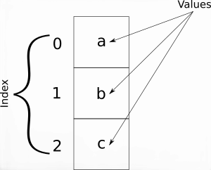
The first main pandas type we will introduce is called Series.
A Series is a single column of data, with row labels for each observation.
pandas refers to the row labels as the index of the Series.
Below, we create a Series which contains the US unemployment rate every other year starting in 1995.
values = [5.6, 5.3, 4.3, 4.2, 5.8, 5.3, 4.6, 7.8, 9.1, 8., 5.7]
years = list(range(1995, 2017, 2))

unemp = pd.Series(data=values, index=years, name="Unemployment")
unemp
1995    5.6
1997    5.3
1999    4.3
2001    4.2
2003    5.8
2005    5.3
2007    4.6
2009    7.8
2011    9.1
2013    8.0
2015    5.7
Name: Unemployment, dtype: float64
We can look at the index and values in our Series.
unemp.index
Index([1995, 1997, 1999, 2001, 2003, 2005, 2007, 2009, 2011, 2013, 2015], dtype='int64')
unemp.values
array([5.6, 5.3, 4.3, 4.2, 5.8, 5.3, 4.6, 7.8, 9.1, 8. , 5.7])
What Can We Do with a Series object?#
.head and .tail#
Often, our data will have many rows, and we won’t want to display it all at once.
The methods .head and .tail show rows at the beginning and end
of our Series, respectively.
unemp.head()
1995    5.6
1997    5.3
1999    4.3
2001    4.2
2003    5.8
Name: Unemployment, dtype: float64
unemp.tail()
2007    4.6
2009    7.8
2011    9.1
2013    8.0
2015    5.7
Name: Unemployment, dtype: float64
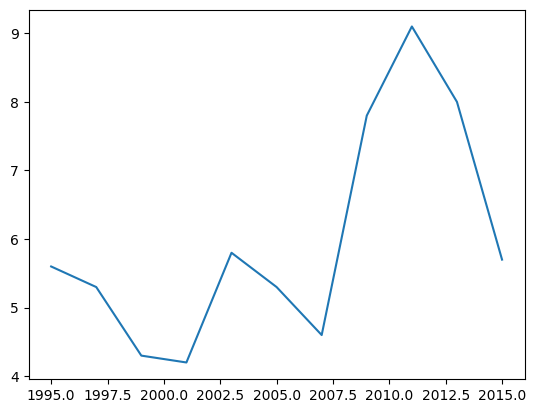
Basic Plotting#
We can also plot data using the .plot method.
unemp.plot()
<Axes: >
Note
This is why we needed the %matplotlib inline — it tells the notebook
to display figures inside the notebook itself. Also, pandas has much greater visualization functionality than this, but we will study that later on.
Unique Values#
Though it doesn’t make sense in this data set, we may want to find the
unique values in a Series – which can be done with the .unique method.
unemp.unique()
array([5.6, 5.3, 4.3, 4.2, 5.8, 4.6, 7.8, 9.1, 8. , 5.7])
Indexing#
Sometimes, we will want to select particular elements from a Series.
We can do this using .loc[index_items]; where index_items is
an item from the index, or a list of items in the index.
We will see this more in-depth in a coming lecture, but for now, we demonstrate how to select one or multiple elements of the Series.
unemp.loc[1995]
5.6
unemp.loc[[1995, 2005, 2015]]
1995    5.6
2005    5.3
2015    5.7
Name: Unemployment, dtype: float64
Exercise
See exercise 1 in the exercise list.
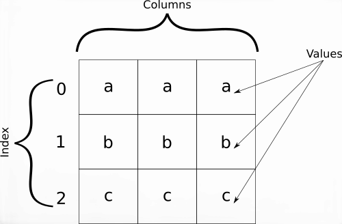
DataFrame#
A DataFrame is how pandas stores one or more columns of data.
We can think a DataFrames a multiple Series stacked side by side as columns.
This is similar to a sheet in an Excel workbook or a table in a SQL database.
In addition to row labels (an index), DataFrames also have column labels.
We refer to these column labels as the columns or column names.
Below, we create a DataFrame that contains the unemployment rate every other year by region of the US starting in 1995.
data = {
    "NorthEast": [5.9,  5.6,  4.4,  3.8,  5.8,  4.9,  4.3,  7.1,  8.3,  7.9,  5.7],
    "MidWest": [4.5,  4.3,  3.6,  4. ,  5.7,  5.7,  4.9,  8.1,  8.7,  7.4,  5.1],
    "South": [5.3,  5.2,  4.2,  4. ,  5.7,  5.2,  4.3,  7.6,  9.1,  7.4,  5.5],
    "West": [6.6, 6., 5.2, 4.6, 6.5, 5.5, 4.5, 8.6, 10.7, 8.5, 6.1],
    "National": [5.6, 5.3, 4.3, 4.2, 5.8, 5.3, 4.6, 7.8, 9.1, 8., 5.7]
}

unemp_region = pd.DataFrame(data, index=years)
unemp_region
| NorthEast | MidWest | South | West | National | |
|---|---|---|---|---|---|
| 1995 | 5.9 | 4.5 | 5.3 | 6.6 | 5.6 |
| 1997 | 5.6 | 4.3 | 5.2 | 6.0 | 5.3 |
| 1999 | 4.4 | 3.6 | 4.2 | 5.2 | 4.3 |
| 2001 | 3.8 | 4.0 | 4.0 | 4.6 | 4.2 |
| 2003 | 5.8 | 5.7 | 5.7 | 6.5 | 5.8 |
| 2005 | 4.9 | 5.7 | 5.2 | 5.5 | 5.3 |
| 2007 | 4.3 | 4.9 | 4.3 | 4.5 | 4.6 |
| 2009 | 7.1 | 8.1 | 7.6 | 8.6 | 7.8 |
| 2011 | 8.3 | 8.7 | 9.1 | 10.7 | 9.1 |
| 2013 | 7.9 | 7.4 | 7.4 | 8.5 | 8.0 |
| 2015 | 5.7 | 5.1 | 5.5 | 6.1 | 5.7 |
We can retrieve the index and the DataFrame values as we did with a Series.
unemp_region.index
Index([1995, 1997, 1999, 2001, 2003, 2005, 2007, 2009, 2011, 2013, 2015], dtype='int64')
unemp_region.values
array([[ 5.9,  4.5,  5.3,  6.6,  5.6],
       [ 5.6,  4.3,  5.2,  6. ,  5.3],
       [ 4.4,  3.6,  4.2,  5.2,  4.3],
       [ 3.8,  4. ,  4. ,  4.6,  4.2],
       [ 5.8,  5.7,  5.7,  6.5,  5.8],
       [ 4.9,  5.7,  5.2,  5.5,  5.3],
       [ 4.3,  4.9,  4.3,  4.5,  4.6],
       [ 7.1,  8.1,  7.6,  8.6,  7.8],
       [ 8.3,  8.7,  9.1, 10.7,  9.1],
       [ 7.9,  7.4,  7.4,  8.5,  8. ],
       [ 5.7,  5.1,  5.5,  6.1,  5.7]])
What Can We Do with a DataFrame?#
Pretty much everything we can do with a Series.
.head and .tail#
As with Series, we can use .head and .tail to show only the
first or last n rows.
unemp_region.head()
| NorthEast | MidWest | South | West | National | |
|---|---|---|---|---|---|
| 1995 | 5.9 | 4.5 | 5.3 | 6.6 | 5.6 |
| 1997 | 5.6 | 4.3 | 5.2 | 6.0 | 5.3 |
| 1999 | 4.4 | 3.6 | 4.2 | 5.2 | 4.3 |
| 2001 | 3.8 | 4.0 | 4.0 | 4.6 | 4.2 |
| 2003 | 5.8 | 5.7 | 5.7 | 6.5 | 5.8 |
unemp_region.tail(3)
| NorthEast | MidWest | South | West | National | |
|---|---|---|---|---|---|
| 2011 | 8.3 | 8.7 | 9.1 | 10.7 | 9.1 |
| 2013 | 7.9 | 7.4 | 7.4 | 8.5 | 8.0 |
| 2015 | 5.7 | 5.1 | 5.5 | 6.1 | 5.7 |
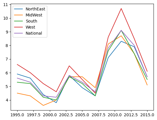
Plotting#
We can generate plots with the .plot method.
Notice we now have a separate line for each column of data.
unemp_region.plot()
<Axes: >
Indexing#
We can also do indexing using .loc.
This is slightly more advanced than before because we can choose subsets of both row and columns.
unemp_region.loc[1995, "NorthEast"]
5.9
unemp_region.loc[[1995, 2005], "South"]
1995    5.3
2005    5.2
Name: South, dtype: float64
unemp_region.loc[1995, ["NorthEast", "National"]]
NorthEast    5.9
National     5.6
Name: 1995, dtype: float64
unemp_region.loc[:, "NorthEast"]
1995    5.9
1997    5.6
1999    4.4
2001    3.8
2003    5.8
2005    4.9
2007    4.3
2009    7.1
2011    8.3
2013    7.9
2015    5.7
Name: NorthEast, dtype: float64
# `[string]` with no `.loc` extracts a whole column
unemp_region["MidWest"]
1995    4.5
1997    4.3
1999    3.6
2001    4.0
2003    5.7
2005    5.7
2007    4.9
2009    8.1
2011    8.7
2013    7.4
2015    5.1
Name: MidWest, dtype: float64
Computations with Columns#
pandas can do various computations and mathematical operations on columns.
Let’s take a look at a few of them.
# Divide by 100 to move from percent units to a rate
unemp_region["West"] / 100
1995    0.066
1997    0.060
1999    0.052
2001    0.046
2003    0.065
2005    0.055
2007    0.045
2009    0.086
2011    0.107
2013    0.085
2015    0.061
Name: West, dtype: float64
# Find maximum
unemp_region["West"].max()
10.7
# Find the difference between two columns
# Notice that pandas applies `-` to _all rows_ at once
# We'll see more of this throughout these materials
unemp_region["West"] - unemp_region["MidWest"]
1995    2.1
1997    1.7
1999    1.6
2001    0.6
2003    0.8
2005   -0.2
2007   -0.4
2009    0.5
2011    2.0
2013    1.1
2015    1.0
dtype: float64
# Find correlation between two columns
unemp_region.West.corr(unemp_region["MidWest"])
0.9006381255384481
# find correlation between all column pairs
unemp_region.corr()
| NorthEast | MidWest | South | West | National | |
|---|---|---|---|---|---|
| NorthEast | 1.000000 | 0.875654 | 0.964415 | 0.967875 | 0.976016 |
| MidWest | 0.875654 | 1.000000 | 0.951379 | 0.900638 | 0.952389 |
| South | 0.964415 | 0.951379 | 1.000000 | 0.987259 | 0.995030 |
| West | 0.967875 | 0.900638 | 0.987259 | 1.000000 | 0.981308 |
| National | 0.976016 | 0.952389 | 0.995030 | 0.981308 | 1.000000 |
Exercise
See exercise 2 in the exercise list.
Data Types#
We asked you to run the commands unemp.dtype and
unemp_region.dtypes and think about the outputs.
You might have guessed that they return the type of the values inside each column.
Occasionally, you might need to investigate what types you have in your DataFrame when an operation isn’t behaving as expected.
unemp.dtype
dtype('float64')
unemp_region.dtypes
NorthEast    float64
MidWest      float64
South        float64
West         float64
National     float64
dtype: object
DataFrames will only distinguish between a few types.
Booleans (
bool)Floating point numbers (
float64)Integers (
int64)Dates (
datetime) — we will learn this soonCategorical data (
categorical)Everything else, including strings (
object)
In the future, we will often refer to the type of data stored in a
column as its dtype.
Let’s look at an example for when having an incorrect dtype can
cause problems.
Suppose that when we imported the data the South column was
interpreted as a string.
str_unemp = unemp_region.copy()
str_unemp["South"] = str_unemp["South"].astype(str)
str_unemp.dtypes
NorthEast    float64
MidWest      float64
South         object
West         float64
National     float64
dtype: object
Everything looks ok…
str_unemp.head()
| NorthEast | MidWest | South | West | National | |
|---|---|---|---|---|---|
| 1995 | 5.9 | 4.5 | 5.3 | 6.6 | 5.6 |
| 1997 | 5.6 | 4.3 | 5.2 | 6.0 | 5.3 |
| 1999 | 4.4 | 3.6 | 4.2 | 5.2 | 4.3 |
| 2001 | 3.8 | 4.0 | 4.0 | 4.6 | 4.2 |
| 2003 | 5.8 | 5.7 | 5.7 | 6.5 | 5.8 |
But if we try to do something like compute the sum of all the columns, we get unexpected results…
str_unemp.sum()
NorthEast                                 63.7
MidWest                                   62.0
South        5.35.24.24.05.75.24.37.69.17.45.5
West                                      72.8
National                                  65.7
dtype: object
This happened because .sum effectively calls + on all rows in
each column.
Recall that when we apply + to two strings, the result is the two
strings concatenated.
So, in this case, we saw that the entries in all rows of the South column were stitched together into one long string.
Changing DataFrames#
We can change the data inside of a DataFrame in various ways:
Adding new columns
Changing index labels or column names
Altering existing data (e.g. doing some arithmetic or making a column of strings lowercase)
Some of these “mutations” will be topics of future lectures, so we will only briefly discuss a few of the things we can do below.
Creating New Columns#
We can create new data by assigning values to a column similar to how we assign values to a variable.
In pandas, we create a new column of a DataFrame by writing:
df["New Column Name"] = new_values
Below, we create an unweighted mean of the unemployment rate across the four regions of the US — notice that this differs from the national unemployment rate.
unemp_region["UnweightedMean"] = (unemp_region["NorthEast"] +
                                  unemp_region["MidWest"] +
                                  unemp_region["South"] +
                                  unemp_region["West"])/4
unemp_region.head()
| NorthEast | MidWest | South | West | National | UnweightedMean | |
|---|---|---|---|---|---|---|
| 1995 | 5.9 | 4.5 | 5.3 | 6.6 | 5.6 | 5.575 |
| 1997 | 5.6 | 4.3 | 5.2 | 6.0 | 5.3 | 5.275 |
| 1999 | 4.4 | 3.6 | 4.2 | 5.2 | 4.3 | 4.350 |
| 2001 | 3.8 | 4.0 | 4.0 | 4.6 | 4.2 | 4.100 |
| 2003 | 5.8 | 5.7 | 5.7 | 6.5 | 5.8 | 5.925 |
Changing Values#
Changing the values inside of a DataFrame should be done sparingly.
However, it can be done by assigning a value to a location in the DataFrame.
df.loc[index, column] = value
unemp_region.loc[1995, "UnweightedMean"] = 0.0
unemp_region.head()
| NorthEast | MidWest | South | West | National | UnweightedMean | |
|---|---|---|---|---|---|---|
| 1995 | 5.9 | 4.5 | 5.3 | 6.6 | 5.6 | 0.000 |
| 1997 | 5.6 | 4.3 | 5.2 | 6.0 | 5.3 | 5.275 |
| 1999 | 4.4 | 3.6 | 4.2 | 5.2 | 4.3 | 4.350 |
| 2001 | 3.8 | 4.0 | 4.0 | 4.6 | 4.2 | 4.100 |
| 2003 | 5.8 | 5.7 | 5.7 | 6.5 | 5.8 | 5.925 |
Renaming Columns#
We can also rename the columns of a DataFrame, which is helpful because the names that sometimes come with datasets are unbearable…
For example, the original name for the North East unemployment rate
given by the Bureau of Labor Statistics was LASRD910000000000003…
They have their reasons for using these names, but it can make our job difficult since we often need to type it repeatedly.
We can rename columns by passing a dictionary to the rename method.
This dictionary contains the old names as the keys and new names as the values.
See the example below.
names = {"NorthEast": "NE",
         "MidWest": "MW",
         "South": "S",
         "West": "W"}
unemp_region.rename(columns=names)
| NE | MW | S | W | National | UnweightedMean | |
|---|---|---|---|---|---|---|
| 1995 | 5.9 | 4.5 | 5.3 | 6.6 | 5.6 | 0.000 |
| 1997 | 5.6 | 4.3 | 5.2 | 6.0 | 5.3 | 5.275 |
| 1999 | 4.4 | 3.6 | 4.2 | 5.2 | 4.3 | 4.350 |
| 2001 | 3.8 | 4.0 | 4.0 | 4.6 | 4.2 | 4.100 |
| 2003 | 5.8 | 5.7 | 5.7 | 6.5 | 5.8 | 5.925 |
| 2005 | 4.9 | 5.7 | 5.2 | 5.5 | 5.3 | 5.325 |
| 2007 | 4.3 | 4.9 | 4.3 | 4.5 | 4.6 | 4.500 |
| 2009 | 7.1 | 8.1 | 7.6 | 8.6 | 7.8 | 7.850 |
| 2011 | 8.3 | 8.7 | 9.1 | 10.7 | 9.1 | 9.200 |
| 2013 | 7.9 | 7.4 | 7.4 | 8.5 | 8.0 | 7.800 |
| 2015 | 5.7 | 5.1 | 5.5 | 6.1 | 5.7 | 5.600 |
unemp_region.head()
| NorthEast | MidWest | South | West | National | UnweightedMean | |
|---|---|---|---|---|---|---|
| 1995 | 5.9 | 4.5 | 5.3 | 6.6 | 5.6 | 0.000 |
| 1997 | 5.6 | 4.3 | 5.2 | 6.0 | 5.3 | 5.275 |
| 1999 | 4.4 | 3.6 | 4.2 | 5.2 | 4.3 | 4.350 |
| 2001 | 3.8 | 4.0 | 4.0 | 4.6 | 4.2 | 4.100 |
| 2003 | 5.8 | 5.7 | 5.7 | 6.5 | 5.8 | 5.925 |
We renamed our columns… Why does the DataFrame still show the old column names?
Many pandas operations create a copy of your data by default to protect your data and prevent you from overwriting information you meant to keep.
We can make these operations permanent by either:
Assigning the output back to the variable name
df = df.rename(columns=rename_dict)Looking into whether the method has an
inplaceoption. For example,df.rename(columns=rename_dict, inplace=True)
Setting inplace=True will sometimes make your code faster
(e.g. if you have a very large DataFrame and you don’t want to copy all
the data), but that doesn’t always happen.
We recommend using the first option until you get comfortable with pandas because operations that don’t alter your data are (usually) safer.
names = {"NorthEast": "NE",
         "MidWest": "MW",
         "South": "S",
         "West": "W"}

unemp_shortname = unemp_region.rename(columns=names)
unemp_shortname.head()
| NE | MW | S | W | National | UnweightedMean | |
|---|---|---|---|---|---|---|
| 1995 | 5.9 | 4.5 | 5.3 | 6.6 | 5.6 | 0.000 |
| 1997 | 5.6 | 4.3 | 5.2 | 6.0 | 5.3 | 5.275 |
| 1999 | 4.4 | 3.6 | 4.2 | 5.2 | 4.3 | 4.350 |
| 2001 | 3.8 | 4.0 | 4.0 | 4.6 | 4.2 | 4.100 |
| 2003 | 5.8 | 5.7 | 5.7 | 6.5 | 5.8 | 5.925 |
Exercises#
Exercise 1#
For each of the following exercises, we recommend reading the documentation for help.
Display only the first 2 elements of the Series using the
.headmethod.Using the
plotmethod, make a bar plot.Use
.locto select the lowest/highest unemployment rate shown in the Series.Run the code
unemp.dtypebelow. What does it give you? Where do you think it comes from?
Exercise 2#
For each of the following, we recommend reading the documentation for help.
Use introspection (or google-fu) to find a way to obtain a list with all of the column names in
unemp_region.Using the
plotmethod, make a bar plot. What does it look like now?Use
.locto select the the unemployment data for theNorthEastandWestfor the years 1995, 2005, 2011, and 2015.Run the code
unemp_region.dtypesbelow. What does it give you? How does this compare withunemp.dtype?